Chapter 15: Molecular Dynamics with GROMACS

This chapter provides a brief overview of using the molecular dynamics simulations with GROMACS, starting from PDB file manipulation. For detailed instructions and the latest features, please consult the official : GROMACS USER MANUAL .

1.1 Introduction

The CHARMM-GUI (Chemistry at HARvard Macromolecular Mechanics Graphical User Interface) is a web-based platform designed for building complex molecular systems and preparing input files for various molecular dynamics software packages, including CHARMM, NAMD, GROMACS, AMBER, OpenMM, GENESIS, and LAMMPS. It simplifies the setup of molecular dynamics simulations, allowing users to quickly configure simulations, including tasks such as introducing point mutations, creating deletions, and setting up steering experiments.

CHARMM-GUI offers an intuitive interface that streamlines the interaction with molecular dynamics software. It is designed to be accessible to both new and experienced users, enabling the execution of both basic and advanced simulations. The platform supports a wide range of simulation techniques, from membrane protein modeling and solvation to free energy calculations and coarse-grained modeling. CHARMM-GUI is a valuable tool for researchers, particularly those without extensive programming experience, facilitating various aspects of molecular dynamics simulations. There are many key features and functionalities are avilable in CHARMM-GUI, however, we will focus on features that are relevant for computational studies of biomolecules include:

i. Input File Generation: CHARMM-GUI generates input files compatible with various molecular dynamics software packages, including CHARMM, NAMD, GROMACS, AMBER, and LAMMPS. It ensures consistency and compatibility between the system setup and the chosen simulation software. ii. System Setup: CHARMM-GUI facilitates the setup of molecular systems by providing tools to build and solvate biomolecular system, including proteins, nucleic acids, lipids, and small molecules. Users can define force fields and customize system parameters such as size, shape, and composition. in preparing input files for molecular dynamics simulations. iii. Force Field Assignment: CHARMM-GUI allows users to assign appropriate force fields and parameters to biomolecular systems, ensuring accurate representation of molecular interactions during simulations. It supports a wide range of force fields compatible with popular molecular dynamics software packages. iv. Solvation and Ionization: The platform assists users in solvating biomolecular systems in explicit solvent environments, with options for adding ions to neutralize system charges and achieve desired ionic strength. It supports various solvent models and provides control over solvation parameters. v. Membrane Builder: It includes specialized tools for constructing lipid bilayers and other membrane systems, essential for simulating biomolecules in realistic cellular environments. Users can specify lipid types, membrane dimensions, and membrane-protein interactions. vi. Ligand Reader and Modeler: CHARMM-GUI can handle the preparation of ligand structures and their integration into the simulation system. vi. Simulation Protocols: CHARMM-GUI offers pre-defined simulation protocols for equilibration and production runs, covering a range of simulation techniques such as molecular dynamics, Monte Carlo simulations, and replica exchange methods. Users can customize simulation parameters and protocols to suit their specific research needs. vii. Advanced Simulation Options: Advanced features include support for enhanced sampling techniques like umbrella sampling, steered molecular dynamics, and free energy calculations. Users can set up complex simulation setups, including multiple replicas, restraints, and analysis options. ix. Analysis Tools: After completing simulations, CHARMM-GUI provides tools for analyzing simulation trajectories, extracting key observables, and visualizing molecular structures and dynamics. It supports a range of analysis techniques, including RMSD analysis, energy calculations, and trajectory visualization.

Overall, CHARMM-GUI serves as a valuable resource for researchers in the field of molecular dynamics, allowing them to set up and analyze simulations efficiently without requiring an in-depth knowledge of the underlying computational methods and protocols. The following sections describe each section in details.

1.2 Loading GROMACS

After installing the GROMACS successfully, typically gmx can be check using following the command

• source /usr/local/gromacs/bin/GMXRC - To load the gmx to your bash shell
• source /home/siu85xxx/gromacs-2022.1/bin/GMXRC - To load the gmx to your bash shell from HPC after installing using miniconda.
• ` gmx help or gmx -h`- provide the current installed version of GROMACS in your system.

gmx can be activate through source /home/siu85xxx/gromacs-2022.1/bin/GMXRC when we are running in the command prompt. However, if we are using the bash script to use source /home/siu85xxx/gromacs-2022.1/bin/gmx to gromacs simulation

1.3 MD Analysis of Protein

In this section, we will investigate the hen egg white lysozyme (PDB code 1AKI), which can be download from RCSB Protein Data Bank. It is recommended check the strcuture using visulization like ChimeraX

1.3.1 Prepare the Molecule for MD

The following are the typical steps for preparing a molecule for MD simulation using GROMACS:

1. Removing Crystal Water:Before proceeding with the simulation, crystal water molecules (HOH) must be removed to avoid unwanted interactions. You can use command-line tools, text editors, or software like ChimeraX.. Avoid using word processing software, as it may alter the file format.
   • grep -v HOH 1aki.pdb > 1AKI_clean.pdb - To remove water molecules using the command line.
2. Generate Molecular Topology Using pdb2gmx: The topology file serves as a blueprint for the simulation, defining atomic interactions, bonding parameters, and force field information.

Missing or incorrect information in the PDB file can cause errors during topology generation using pdb2gmx and may compromise the simulation.

• Common Issues That May Cause pdb2gmx to Fail:
  • Missing atoms: Missing atoms within residues will lead to errors.
  • Missing residues: Look for lines with “MISSING” in the PDB file, indicating incomplete structures.
  • Terminal regions: Ensure “TER” entries are included to mark chain terminations correctly.
  • Incomplete sequences: Some residues may lack atoms, requiring manual correction.
• Limitation of pdb2gmx:
  • Not fully automated: It cannot generate topologies for arbitrary molecules (e.g., ligands or complex cofactors).
  • Restricted residue support: Works primarily with standard biomolecules (proteins, nucleic acids, some cofactors like NAD(H), ATP).
  • Missing atoms/residues must be fixed before running pdb2gmx.

After removing water, verify that all necessary atoms are present in the PDB file before proceeding. Next, generate the molecular topology and structure file using the GROMACS pdb2gmx module:

Upon execution of the following commands, GROMACS will prompt you to choose a force field. Select: 15: OPLS-AA/L all-atom force field (2001 aminoacid dihedrals)

• gmx pdb2gmx -f 1AKI_clean.pdb -o 1AKI_processed.gro -water spce

Or we can specific the output of topol and posre file name with following commands.

gmx pdb2gmx -f 1AKI_clean.pdb -p topol.top -i posre.itp -o 1AKI_processed.gro -water spce .

Running pdb2gmx creates three key file:

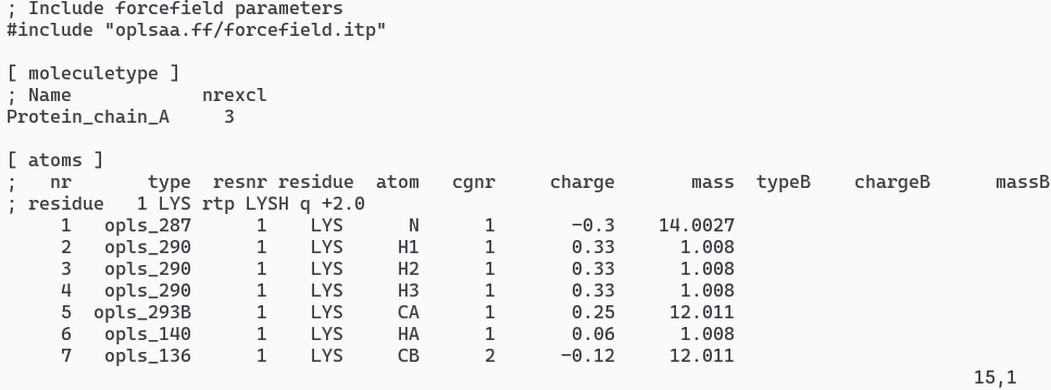
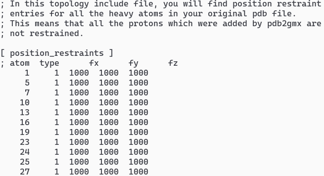
1. Topology file (.top): Defines molecules, atoms , force field parameters. It contains nonbonded (atom types, charges) and bonded parameters (bonds, angles, dihedrals). Defines molecular interactions according to the chosen force field.
2. Position restraint file (posre.itp): Used for restraining atoms (typically heavy atoms) during equilibration to prevent large movements.
3. Processed structure file (.gro): (A GROMACS) structure file with atomic positions and velocities. The .gro files is not mandatory, GROMACS supports multiple formats, including PDB (.pdb). If you prefer using the PDB format, simply specify the output filename with a pdbextension.

Typical output of topology file"

Information about the water model can be found at Water Sctructure and Science .

Examine the Topology and restraints file using text file. You can find various comments and sections [atoms], [bonds], [pairs], [angles], and [dihedrals].

• vi totp.top - Typical output of topology is shown in Figure 1
• vi posre.itp - Typical output of restrain is shown in Figure 1

Typical output of position restrain file"

1.3.2 Common Water Models in GROMACS

Depending on your installed force fields, the following water models are typically available in GROMACS:

• ls /usr/local/gromacs/share/gromacs/top/ - list available water models in the force field directory. Inside this directory, the .itp files (e.g., spce.itp, tip3p.itp) correspond to available water models.

topology file must match molecular order with .gro. The names list must match the [ moleculetype ] name for each species, not residue names or anything else.

1. Create Box and Solvate: We will follow two steps There are two steps: i. defining the box dimensions using gmx editconf module: Highly recommend the rhombic dodecahedron, as its volume ~71% of cubic box of same periodic distance, thus saving on number of water molecules that need to be added to solvate the protein.

• gmx editconf -f 1AKI_processed.gro -o 1AKI_newbox.gro -c -d 1.0 -bt cubic

filling the box using solvate module (formerly called genbox): -c: center molecule in box, and -d 1.0: distance between solute and box (at least 1.0 nm from box), -bt cubic: cubix box type. We are using the periodic boundary conditions and protein should never see its periodic image.

ii. We will fill the box with solvent (water) using gmx solvate

• gmx solvate -cp 1AKI_newbox.gro -cs spc216.gro -o 1AKI_solv.gro -p topol.top

-cp: configuration of protein. Filling box with solvent (water). The default solvent is Simple Point Charge water (SPC), with coordinates from spc216.gro, a generic equilibrated 3-point solvent model. We can also use spc216.gro as solvent configuration for SPC, SPC/E, or TIP3P, all are 3-point water models. Keep track of how many water molecules it has added. Note the changes to the [ molecules] directive of topol.top at the end of the file:

[ molecules ] ; Compound #mols Protein_A 1 SOL 10832

Note that if you use any other (non-water) solvent, solvate will not make these changes to your topology! Its compatibility with updating water molecules is hard-coded. For more information, gmx solvate -h in the command line.

1. Energy minimization

• Need visualization xmgrace which can be install by:
• conda install -c conda-forge grace - Using conda-forge (recommended)
• sudo apt-get install grace - Istalling via your system package manager
• xmgrace - to launch emgrace

1. Equilibration in GROMACS Both NVT and NPT equilibration steps are essential in GROMACS (and molecular dynamics in general) to prepare your system for a stable production MD run.

• Step 1: NVT (Constant Number of particles, Volume, and Temperature). The goal is to stabilize the temperature of the system. Here letting the water/ions settle around your molecule while gently heating everything up. The procedue is:
  • Keeps volume fixed.
  • Gradually brings the system to the desired temperature (e.g., 300 K).
  • Removes artifacts from energy minimization (e.g., unrealistic velocities).
  • Applies position restraints to heavy atoms (usually protein) so the solvent can adapt around it. We let the protein, don’t wiggle too much while the solvent finds its groove.

The main reasons restrain Heavy Atoms (= all non-hydrogen atoms), Hydrogen atoms are light and fast-moving anyway, so they’re usually not restrained:

• Prevent large/unrealistic movements of solute atoms during the early stages of equilibration.
• Let the solvent (e.g., water, ions) adjust and relax around a stable solute.
• Avoid artificial distortion or unfolding of biomolecules while temperature or pressure is ramping up.

Especially right after energy minimization, some water or ions may be poorly placed. If the protein moves too freely, things can go wild — leading to simulation crashes or bad dynamics.

During production MD, we usually remove restraints, so the system evolves naturally. Restraints are only meant for the equilibration phase. In .mdp file, we include define = -DPOSRES which tells GROMACS to include the posre.itp file for atoms that are marked as restrained in your topology.

• Step 2: NPT (Constant Number of particles, Pressure, and Temperature). Goal: Stabilize the pressure and let the box size/volume adjust naturally. Here, we are letting the box “breathe” and find its natural size under realistic pressure. The procedue is:
  • Keeps temperature constant (as already stabilized by NVT).
  • Allows box volume to fluctuate so pressure can equilibrate (target: 1 bar).
  • Ensures density and pressure of your system match experimental or physiological conditions.

1. Analysis Step 1 Using gmx trjconv (a pos-processing tool) to remove periodic boundary conditions (PBC) and center your molecule in the simulation box — a common step before visualization or analysis. Let’s break this command down and make sure you run it correctly.
   • gmx trjconv -s md_0_1.tpr -f md_0_1.xtc -o md_0_1_noPBC.xtc -pbc mol -center
   • Flags:
     • s md_0_1.tpr: Structure/topology file (needed for box info and atom groups).
     • f md_0_1.xtc: Original trajectory file (with PBC effects).
     • o md_0_1_noPBC.xtc: Output trajectory (with fixed PBC and centered).
     • pbc mol: Treats molecules as whole units when unwrapping across PBC.
     • center: Centers selected group in the box.

When we run this, GROMACS will ask twice:

1. “Select group for centering:” Choose the group you’d like to center, usually something like: Protein, Backbone, Protein-H, or DNA (if applicable).
2. “Select output group:” Choose the entire system or what you want to output: System, Protein (if you want only the protein), or Protein + solvent, etc.

• gmx rms -s em.tpr -f md_0_1_noPBC.xtc -o rmsd_xtal.xvg -tu ns - calculating RMSD relative to the minimized structure (em.tpr), likely to compare how much your system deviates from the initial crystal or model structure. Solid move, especially if you’re interested in structural stability over time.
  • s em.tpr: Reference structure — your energy-minimized (often crystallographic) structure.
  • f md_0_1_noPBC.xtc: Trajectory with PBC artifacts removed and system centered.
  • o rmsd_xtal.xvg: Output RMSD values over time.
  • tu ns: Report time in nanoseconds (default is picoseconds).

  You’ll be prompted twice:

Group for least-squares fit (alignment)

1. e.g., Protein Group for RMSD calculation
2. e.g., Protein