Appendix

2.1 Chapter 2

2.1.1 Taylor Series and Binomial Expansion

The Taylor series is a powerful tool in mathematics that represents a function as an infinite sum of terms, calculated from the values of its derivatives at a single point. The Taylor series of a function \(f(x)\) about a point \(a\) is given by:

\begin{equation} f(x) = f(a) + f’(a) (x-a) + \frac{f’‘(a)}{2!} (x-a)^2+ \dots \end{equation} this can be writing more compactly as: \begin{equation} f(x) = \sum_{n=0}^{\infty} \frac{f^{(n)}(a)}{n!} (x-a)^n \end{equation} where \(f^{(n)} (a)\) is the n\(^{th}\) derivative of \(f(x)\) evaluated at \(x= a\).

Derivation of the Taylor Series

Let’s assume a function \(f(x)\) can be represented by a power series centered at \(x= a\): \begin{equation} f(x) = c_0 + c_1(x-a) +c_2 (x-a)^2 + c_3 (x-a)^3 + \dots \end{equation} this is equivalent to: \begin{equation} f(x) = \sum_{n=0}^{\infty} c_{(n)} (x-a)^n \end{equation} The goal is to determine the coefficients \(c_n\).

Evaluate at \(x=a\), Substitute \(x =a\) into the power series, \begin{equation} f(a) = c_0 + c_1(a-a) +c_2 (a-a)^2 + c_3 (a-a)^3 + \dots \ \Rightarrow \ c_0 = f(a) \end{equation}

Take the 1\(^{st}\) derivative and evaluate at \(x =a\): \begin{equation} f’(x) = c_1 + 2 c_2 (x-a) + 3 c_3 (x-a)^2 + \dots \end{equation} and substitute \(x =a\): \begin{equation} f’(a) = c_1 \end{equation} Similarly second derivative and evaluate at \(x =a\), we found that \begin{equation} f’‘(a) = 2 c_2 \ \Rightarrow c_2 = \frac{f’‘(a)}{2} \end{equation} continue this process for higher derivatives, the general pattern is \begin{equation} c_n = \frac{f^{(n)}(a)}{n!} \end{equation} Substitute the coefficients back into the series, we obtain the Taylor series \begin{equation} f(x) = \sum_{n=0}^{\infty} \frac{f^{(n)}(a)}{n!} (x-a)^n \end{equation}

Binomial Expansion For any positive integer n, \begin{equation} (x+y)^n = \sum_{k=0}^{n} \binom{n}{k} x^{n-k} y^{k} = x^n + n x^{n-1} y + \dots + n x y^{n-1} + y^n \end{equation} and \begin{equation} (1+x)^n = \sum_{k=0}^{n} \binom{n}{k} x^k = 1 + n x + \frac{n(n-1)}{2!} x2 + \dots + x^n \end{equation} where the binomial coefficient

\begin{equation} \binom{n}{k} =\frac{n!}{k!(n-k)!} \end{equation}

When \(n\) is not a positive integer, the binomial expansion becomes an infinite series, valid for \(|x| \leq 1\): \(\begin{eqnarray} (1+x)^n &=& 1 + n x + \frac{n (n-1)}{2!} x^2 + \dots \\ (1-x)^n & \approx & 1- nx \hspace{1in} \text{for } x \ll 1 \end{eqnarray}\)

6. Chapter 6

6.1 Derivation of Wave Equation

The vibration of strings in musical instruments was extensively studied by several scientists in the 18^th century, including Ernst Chladni and Joseph Sauveur, alongside notable figures like Jean le Rond d’Alembert, Leonhard Euler, Daniel Bernoulli, and Joseph-Louis Lagrange.

A transverse wave on a string.

The one-dimensional wave equation was first derived by the French mathematician Jean le Rond d’Alembert in 1747. His work provided a foundational solution for vibrating strings, known as d’Alembert’s formula. However, the extension to the three-dimensional wave equation is more complex and cannot be solely attributed to Leonhard Euler. While Euler contributed significantly to the field of wave equations, the three-dimensional wave equation is generally expressed as

\[\nabla^2 u - \frac{1}{v^2} \frac{\partial^2 u}{\partial t^2} = 0\]

where \(u\) is the wave function and \(v\) is the wave speed

The wave equation for a transverse wave on a stretched string in one dimension is correctly stated as:

\[\frac{\partial^2 y(x,t)}{\partial t^2} = v^2 \frac{\partial^2 y(x,t)}{\partial x^2}\]

where \(y(x,t)\) represents the transverse displacement of the string at position \(x\) and time \(t\), and \(v\) is the wave propagation speed.

All wave equations, including the wave equation for a vibrating string, are derived from fundamental physical principles, specifically Newton’s second law of motion, \(F=ma\)

A transverse wave on a string.

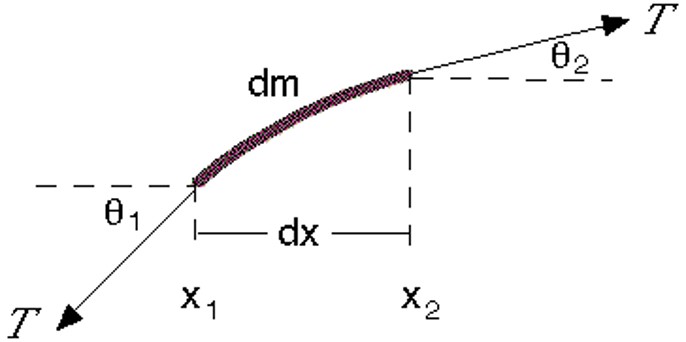
Let’s derive the wave equation using Newton’s second law. Consider a small segment of a string undergoing a traveling wave, as illustrated in Figure 2. We can apply Newton’s second law in the vertical direction:

\[F_y = m a_y\]

The net vertical force acting on the segment can be expressed as:

\[F_y = T \sin \theta_2 - T \sin \theta_1\]

Here, \(T\) is the tension in the string, and \(\theta_1\) and \(\theta_2\) are the angles the string makes with the horizontal at the endpoints of the segment. Using the small angle approximation, we can simplify the sine functions:

\[\sin \theta \approx \tan \theta \approx \frac{\partial y}{\partial x}\]

This approximation holds true when the angles are small, allowing us to relate the angles to the slope of the string. Here, slop is changing over x so the net force is not zero, but for a straight string net force is zero.

Substituting the small angle approximation into our force equation gives:

\[F = T \left(\frac{\partial y}{\partial x}\right)_2 - T \left(\frac{\partial y}{\partial x}\right)_1\]

Next, consider a small mass element \(dm = \mu dx\), where \(mu\) is the mass per unit length. The acceleration in the vertical direction can be expressed using Newton’s second law:

\[F = m a_y\]

Thus, we can write:

\[F = (\mu dx) \frac{\partial^2 y}{\partial t^2}\]

Equating the two expressions for force gives:

\[T \left(\frac{\partial y}{\partial x}\right)_2 - T \left(\frac{\partial y}{\partial x}\right)_1 = (\mu dx) \frac{\partial^2 y}{\partial t^2}\]

Rearranging this equation leads to:

\[\frac{\partial^2 y}{\partial t^2} = (\frac{T}{\mu}) \frac{\left(\frac{\partial y}{\partial x}\right)_2 - \left(\frac{\partial y}{\partial x}\right)_1}{dx}\]

Using the definition of the second derivative, we can express this as:

\[\frac{\partial^2 y}{\partial t^2} = \frac{T}{\mu} \frac{\partial^2 y}{\partial x^2}\]

The general solution to this wave equation is given by:

\[y = A \sin(kx - \omega t)\]

From this solution, we can derive the relationship:

\[\frac{T}{\mu} = \frac{\omega^2}{k^2} = v^2\]

Thus, we arrive at the wave equation:

\[\frac{\partial^2 y}{\partial t^2} = v^2 \frac{\partial^2 y}{\partial x^2}\]

which describes the propagation of waves in a medium with a speed \(v\). Notably, it can be applied to electric and magnetic fields. Although Maxwell’s equations intricately couple the electric and magnetic fields, electromagnetic (EM) waves can be understood as solutions to wave equations: one for the electric field \(E\) and one for the magnetic field \(B\). Both fields satisfy the wave equation, derivable from the fundamental laws of electricity and magnetism.

Consider an EM wave propagating in the x-direction, with the electric field (\(E\)) oscillating along the y-axis and the magnetic field (\(B\)) oscillating along the z-axis. The wave equations for these fields are:

\[\begin{eqnarray} \frac{\partial ^2 E_y}{\partial t^2} &=& c^2 \frac{\partial ^2 E_y}{\partial x^2} \\ \frac{\partial ^2 B_z}{\partial t^2} &=& c^2 \frac{\partial ^2 B_z}{\partial x^2} \end{eqnarray}\]

The solutions for these equations are sinusoidal functions representing the oscillating electric and magnetic fields:

\[\begin{eqnarray} E(x,t) &=& E_m \sin(k x - \omega t)\hat{y} \\ B(x,t)&=& B_m \sin(k x - \omega t)\hat{z} \end{eqnarray}\]

where:

• \(E_m\) and \(B_m\) are the ampliture of the electric and magnetic fields,
• \(k = 2\pi/\lambda\) is the wave number,
• \(\omega = 2\pi f\) is the angular frequency,
• \(c = 1/\sqrt{\mu_0 \varepsilon_0}\) is speed of light in vacuum,
• \(\varepsilon_0 \approx 8.85 \times 10^{-12} F/m\)$ is electric permittivity of free space, and
• \(\mu_0 = 4\pi \times 10^{-7} N/A^2\) is the magnetic permeability of free space.

The relationship between the amplitudes of the electric and magnetic fields is given by:

\[\begin{equation*} \frac{E_m}{B_m} =c \end{equation*}\]

These equations represent the mathematical description of a propagating electromagnetic wave. The electric and magnetic fields oscillate perpendicularly to each other and to the direction of wave propagation, a fundamental property of transverse waves.