Chapter 1: Pre-Modern Physics

Posted Dec 10, 2024 Updated Feb 16, 2025

By Poopalasingam Sivakumar

22 min read

This chapter serves as a guide to outline the key events and concepts in the journey towards modern physics. We belive the significance of comprehending these events before delving into modern physics. Additionally, exploring the history behind these events can help us grasp the evolution, not just the outcomes. However, our review doesn’t replace the fundamentals knowledge covered in an introductory physics course. We assume you are familiar with basic concepts such as vectors, partial derivatives, and integration. This review primarily focuses on essential classical mechanics, particularly classical relativity, serving as a stepping stone for the following chapter. The content presented here is intentionally concise, intended as a quick refresher. For a more in-depth understanding, we encourage revisiting the materials from the introductory physics courses.

1.1 Introduction

The physics has a long and fascinating histroy with many significant discoveries and milestones along the way. Among the most notable milestones before modern physiccs (20^th century), classical mechanics emerged in the 17^th century, primarily attribuated to Isaac Newton, and further enriched by contributions from various mathematicisian and physicist, including Johannes Kepler, Leonhard Euler, Joseph-Louis Lagrange, and others. This theory laid the groundwork for comprehending the motion of objects at macroscopic scales and the laws that govern them. Classical physics remains a vital branch of physics. Another important milestone was the development of thermodynamics in the 19^th century, which helped us understand the relationship between heat, energy, and the principles of entropy.

Finally, the revelation of electromagnetism in the 19^th century. These milestones paved the way for modern physics. The subsequent timeline chart highlisths several major milestones pre-modern physics.

Chronology of Key Milestones in Pre-modern Physics

1564-1642
Galileo Galile
An Italian scholar, studied nature, stars, and mathematics. He is widely regarded as a foundational figure in the advancement of physics. Thanks to his experiments and methods,which have had a profound impact on our understanding of the laws governing the physical world. He is best known for his observations with a telescope, which unveiled groundbreaking astronomical discoveries, including Jupiter's moons and Venus's phases. $\textbf{Galileo}$ is one of the most important figures in the history of science.
1642-1727
Sir Isaac Newton
An English scholar made groundbreaking contributions to science, particularly in physics and mathematics. He formulated the laws of motion and universal gravitation, laying the groundwork for classical mechanics. Additionally, he made significant advancements in calculus, optics, and the study of light and color. His work revolutionized scientific thought, profoundly influencing various fields for centuries to come. Beyond Newtonian mechanics, numerous alternative formulations, including Lagrangian dynamics, Hamilton’s formulation, and the Hamilton-Jacobi theory, have been developed to describe the complexities of motion, expanding upon his foundational work .
1785
Coulomb's Law
It describes the electrostatic force between charged particles, $ F = k \cdot \frac{q_1 \cdot q_2}{r^2} $. It is named after the French physicist $\textbf{Charles-Augustin de Coulomb}$ (1736-1806), who first formulated the law in the late 18^th century.
1811
Avodgadro's law
$\textbf{Amedeo Avogadro}$ (1776-1856)suggested that equal volumes of gases, at the same temperature and pressure, contain an equal number of molecules, regardless of the type of gas. The term "Avogadro number" was later proposed by the French physicist $\textbf{Jean Perrin}$ to honor Avogadro's contributions to the understanding of the molecular nature of gases.
1823
Ampère's Law
$\textbf{André-Marie Ampère}$ (1775-1836), a French physicist and mathematician, related the magnetic field around a closed loop to the electric current passing through the loop, which is called Ampère's Law: $ \oint \mathbf{B} \cdot d\mathbf{\ell} = \mu_0 \iint_S \mathbf{J} \cdot d\mathbf{S} = \mu_0 I_{\text{enc}}$.
1824
Carnot's Theorem
French Military engineer and physicist $\textbf{Nicolas Léonard Sadi Carnot}$ (1796-1832) developed the inaugural theory on the maximum efficiency of heat engines, famously known as Carnot's theorem: any heat engine operating between two heat reservoirs is inherently less efficient than a Carnot heat engine functioning between the same reservoirs.
1831
Faraday's Law
This law$ \mathcal{E} = -\frac{d \phi_B}{dt}$, stating that the electromotive force ($ \mathcal{E}$) induced in a circuit is equal to the negative rate of changes of magnetic flux ($\phi_B$) through the circuit. It was independently discovered by $\textbf{Michael Faraday} $(1791-1867) in 1831 and $\textbf{Joseph Henry}$ (1797-1878) in 1832. However, it was Michael Faraday who first published the results.
1835
Gauss's Law
It relates the electric flux through a closed surface to the total electric charge enclosed by that surface, $ \oint (\mathbf{E} \cdot d\mathbf{A}) = \frac{Q}{\varepsilon_0} $. The law is named after the German mathematician and physicist $\textbf{Carl Friedrich Gauss}$ (1777–1855), who formulated it.
1851
Law of thermodynamics
The formulation of the first and second laws of thermodynamics and the concept of absolute zero temperature are indeed attributed to several scientists, but Lord Kelvin (William Thomson) contributed significantly to the development and understanding of these principles.
1864
Classical Electromagnetism
James Clerk Maxwell (1831-1879) revolutionized the understanding of electricity and magnetism by formulating a set of four fundamental partial differential equations. These equations, known as Maxwell's Equations, describe how electric and magnetic fields interact with matter. His pioneering work not only established that light behaves as an electromagnetic wave but also introduced the idea that these waves travel uniformly. Maxwell's contributions laid the groundwork for a significant part of both modern physics and engineering.
1895
Maxwell-Boltzmann Velocity Distribution
It, defining the spread of speeds within a gas at a given temperature, was formulated through the collaboration of Scottish mathematical physicist $\textbf{James Clerk Maxwell}$ (1831-1879) and Austrian physicist and philosopher $\textbf{Ludwig Eduard Boltzmann}$ (1844-1906). This distribution illustrates how the velocities of gas particles vary within a gas sample, providing crucial insights into statistical mechanics and the behavior of gases at different temperatures.

While classical physics remains highly accurate and applicable in most everyday scenarios and technologies, it encounters limitations in extreme conditions, such as very high speeds (nearing the speed of light, necessitating special relativity) and exceedingly small scales (atomic or subatomic levels, necessitating quantum mechanics). These limitations prompted the development of modern physics, which emerged in the 20^th century and broadened our comprehension of the physical world beyond classical physics’ scope. Although its scope narrows in these extreme conditions, classical mechanics still stands as a vital foundation for comprehending the physical world, paving the way for more advanced branches of physics.

1.2 Review of Classical Mechanics

Classical mechanics is a branch of physics that studies the motion of macroscopic objects. It provides a framework for understanding the motion of objects and the forces that act upon them. The field is based on a set of essential concepts and equations that describe how physical systems work in various conditions. Key concepts include Newton’s laws of motion, conservation of energy, conservation of momentum, and the principle of least action. These concepts help us understand how objects move and the force that affect them.

Newton’s second law connects force and acceleration, while the law of gravitation explains how objects with mass attract each other. Equations of motion describes the trajectory of object using its position, velocity, and acceleration. The Lagrangian equations are another valuable tool, describing a system’ movement based on its energy. These ideas and equaiton are fundamental to clsscical mechanics and are vital for understanding how things work in daily life. The following presents important concepts and equations that are fundamental to classical mechanics.

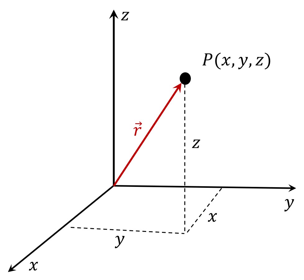
Let’s consider a particle with resepect to the orgin in a Cartesian coordinate system, represented by the positinve vector $\vec{r}$ (refer to Figure 1). The particle’s position can be either positivie, negative, or zero. The position vector can be expressed as follows:

\begin{equation} \vec{r} = x \hat{i} + y\hat{j} + z \hat{k} \tag{1.1} \end{equation}

Description of the image — 3D Cartesian coordinate system.

When a particle moves from position $\vec{r}_1$ to position $\vec{r}_2$ during a time interval $\Delta t = t_2 - t_1$, the average velocity during the inverval is given by

\begin{equation} \vec{v}_{avg} = \frac{\Delta \vec{r}}{\Delta t} = \frac{\vec{r}_2- \vec{r}_1}{t_2-t_1} \tag{1.2} \end{equation}

The average speed of the particle during a time inverval $\Delta t$ depends on the total distance covered in that time interval

\begin{equation} s_{avg} = \frac{\text{total distance}}{\Delta t} \tag{1.3} \end{equation}

For a moving particle, the instantaneous velocity is defined as \begin{equation} \vec{v} = \lim_{\Delta t \leftarrow 0} \frac{\Delta \vec{r}}{\Delta t} = \frac{d \vec{r}}{dt} \tag{1.4} \end{equation} Average acceleration of a particle is the ratio of a change in velocity $\Delta \vec{v}$ to the time interval $\Delta t$ in which the change occurs: $\begin{equation} \vec{a}_{avg} = \frac{\Delta \vec{v}}{\Delta t} = \frac{\vec{v}_2- \vec{v}_1}{t_2-t_1} \tag{1.5} \end{equation}$ The instantaneous acceleration can be expressed as $\begin{equation} \vec{a} = \lim_{\Delta t \leftarrow 0} \frac{\Delta \vec{v}}{\Delta t} = \frac{d \vec{v}}{dt} = \frac{d^2\vec{r}}{dt} \tag{1.6} \end{equation}$ Under the constant acceleration, the following equations describe the motion of a particle.

\[\begin{eqnarray} \vec{v} &=& \vec{v}_0 + \vec {a} t \tag{1.7} \\ \vec{r} &=& \vec{r}_0 + \vec{v}_0 t + \frac{1}{2} \vec{a} t^2 \nonumber \\ \vec{v}^2 &=& \vec{v}^2_0 + 2 \vec{a} (\vec{r} - \vec{r}_0) \nonumber \\ \vec{r} &=& \vec{r}_0 + \frac{1}{2} (\vec{v}_0 + \vec{v}) t \nonumber \\ \end{eqnarray}\]

$\textbf{Particle in Uniform Circular Motion}$: Imagine a particle that moves around a circle with a fixed radius r and a constant speed $v$. The particle’s acceleration $a$, known as centripetral acceleration, is always towards the center of the circle and is perpendicualr to its velocity $\vec{v}$. The magnitude of this acceleration is given by,

\[\begin{equation} a_c = \frac{v^2}{r} \tag{1.8} \end{equation}\]

The period of the particle’s motion, denoted by T, is expressed as $\begin{equation} T = \frac{2\pi r}{v} \tag{1.9} \end{equation}$ The angular speed $\omega$ of the particle is given as

\[\begin{equation} \omega = \frac{2\pi}{T} \tag{1.10} \end{equation}\]

The main role in classical mechanics, describes the motion of macroscopic objects at speeds much slower than the speed of light, is Newton’s laws of motion, which are:

$\textbf{Newton's First Law (Law of Inertia)}$: An object at rest stays at rest, and an object in motion continues in motion with a constant velocity unless acted on by a net external force.
$\textbf{Newton's Second Law}$: The acceleration of an object is directly proportional to the net external force acting on it and inversely proportional to its mass. Newton’s second law can be expressed mathematically as,

\begin{equation} \vec{a} \propto \frac{\sum{\vec{F}}}{m} \Rightarrow \ \sum{\vec{F}} = m \vec{a} \tag{1.11} \end{equation}

The SI unit of foce is the newton (N), where $1\ N = 1\ kg \cdot m/s^2$.

$\textbf{Newton's Third Law}$: For every action, there is an equal and opposite reaction. This law highlights the symmetry of forces in nature. Newton’s third law is expressed mathematically,

\begin{equation} \vec{F}{12} = - \vec{F}{21} \tag{1.12} \end{equation}

$\textbf{Work done by a constant force}$: If a constant force $\vec{F}$ acts on a particle that displaces a straight-line $\Delta \vec{r}$. The work done by the force on the particle is

\begin{equation} W = \vec{F} \cdot \Delta \vec{r} = F \Delta r \cos \theta \tag{1.13} \end{equation}

$\textbf{Work done by a varying force or on a curved path}$ When a force that varies with position or a curved path, the work is generally expressed as the line integral of a varying force over an arbitrary path. It is given by \begin{equation} W = \int dW = \int \vec{F} \cdot d\vec{r} \tag{1.14} \end{equation} The unit of work in SI units is the joule (J), and $1 \ J = 1 \ N \cdot m = 1 kg \cdot m^2/s^2$.

$\textbf{Kinetic Energy}$: Kinetic energy is the energy linked to the motion of an object. The kinetic energy (KE) is a scalar quantity and is defined by the expression: \begin{equation} K.E = \int F_x dx = \int m \frac{dv}{dt} dx = \int (m v)\ dv = \frac{1}{2} m v^2 \tag{1.15} \end{equation} where m is mass and $v$ is the speed of the object. The unit of energy in SI units is the joule (J), and $1 J = 1\ N \cdot m = 1 \ kg \cdot m^2/s^2$.

$\textbf{Potential Energy}$: Associated with the position or configuration on an object, potential energy is a form of energy that an object possesses because of it relative position or state. It explains the behavior of systems, and provides insights into the transformation between different forms of energy in physical processes. The two most common types of potential energy are gravitational potential energy and elastic potential energy.

i. $\textbf{Gravitational Potential Energy}$: the Gravitational potential energy is associated with an object’s position in a gravitational field. The work done on an object by a constant gravitational force ($F_g = mg$) can be illustrated as a change in the gravitational potential energy, given by the expression $\begin{equation} \Delta U_g = U_f - U_i = - \int_{y_i}^{y_f} (-mg) \ dy = mg\ (y_f - y_i) \tag{1.16} \end{equation}$

where m is the mass of the object, g is the acceleration due to gravity, and $y_i$ and $y_f$ are inital and final height of the object.

ii. $\textbf{Elastic Potential Energy}$: This is associated with the elastic force resulting from the stretching or compressing of elastic materials like springs. The elastic force, generated when the material is diplaced by a distance (x) from its equilibrium position, is given by Hooke’s Law: $\begin{equation} F_e = - kx \tag{1.17} \end{equation}$ Here, k represents the spring constant. The change of potnetial energy of elastic system: \begin{equation} \Delta U_e = U_f - U_i = - \int_{x_i}^{x_f} (-kx) dx = \frac{1}{2} k (x_f^2 - x_i^2) \tag{1.18} \end{equation}

where the unit of energy is $Jule \ (J) = kg \cdot m^2/s^2$. If the potential energy function $U(x)$ for a system is known, the force (F(x)) can be determined using the expression: \begin{equation} F(x) = - \frac{dU(x)}{dx} \tag{1.19} \end{equation}

$\textbf{Linear Momentum}$: The linear momentum is a fundamental concepts that describes the motion. It is the product of an object’s mass (m) and its velocity ($\vec{v}$) and is a vector quantity. It is mathematically expressed as: \begin{equation} \vec{p} = m \vec{v} \tag{1.20} \end{equation} According to Newton’s second law, the rate change of momentum of an object is equal to the net force acting on it. This relationship is expressed as \begin{equation} \vec{F} = \frac{d \vec{p}}{dt} \tag{1.21} \end{equation} One can notice that in an isolated system where no external forces are acting, the principle of conservation of linear momentum states that the total linear momentum of the system remains constant $\Delta \vec{p} = 0$.

$\textbf{Impulse}$, is a fundamental concept, plays a crucial role in understanding and analyzing interaction between objects, particularly during collisions. It offers valuable insights into how forces influence the motion of objects. Impulse, a vector quantity, is expressed as the integral of net force acting on an object over a given time inteval \begin{equation} \vec{I} = \int_{t_1}^{t_2} \sum{\vec{F}}dt \tag{1.22}
\end{equation}

If $\vec{F}_{avg}$ represents the average force of $\vec{F}(t)$ during the collision, and $\Delta t$ is the duration of the collision, then the impulse can be expressed as: \begin{equation} I = \vec{F}_{avg} \Delta t \tag{1.23} \end{equation} It is closely linked to the change in momentum of an object, represented as
\begin{equation} \vec{I} = \Delta \vec{p} \tag{1.24} \end{equation}

$\textbf{Torque}$ also referred as the “rotational force” that describe the rotational force or the tendency to cause an object to rotate about an axis. The torque is defined as the corss product of the radius vector $\vec{r}$ from a given axis to the point where a force $\vec{F} is applied \begin{equation} \vec(\tau) = \vec{r} \times \vec{F} \tag{1.25} \end{equation}

$\textbf{Angular Momentu}$ is a fundamental concept in physics that describes the rotational motion of an object. The angular momentum of a point particle with respect to point O is defineds as \begin{equation} \vec{L} = \vec{r} \ \times \vec{p} = \vec{r} \ \times \ m \vec{v} \tag{1.26} \end{equation} Here, $\vec{r}$ is the position vector from the particle to point O and $\vec{p}$ is the linear momentum. When a body rotates about an axis, the angular mementum is expressed as: \begin{equation} \vec{L} = I \vec{\omega} \tag{1.27} \end{equation} where I is the momentum of intertia of the object about the axis of rotation, and $\vec{\omega}$ is the angular velocity.

The net external torque $(\sum \vec{\tau})$ on a system is equal to the rate of change of its angular momentum: \begin{equation} \sum \vec{\tau} = \frac{d\vec{L}}{dt} \tag{1.28} \end{equation}

In the next section, we will delve into the fundamental concepts of in classical mechanics.

1.3 Classical Relativity

Before introducing special relativity in the next chapter, it is important to establish the fundamentals of relativity itself. This involves understanding the Galilean transformation, which describes the relationship between coordinates in inertial reference frames. The fundamental concept of relativity, maintaining the same form across various reference frames, can be traced back to the contributions of Galileo Galilei and Isaac Newton in classical mechanics.

Galileo Galilei introduced the concept of relative motion and demontrated that the laws of physics are the same in all inertial reference frames within the framework of classical mechanics. Isaac Newton, on the other hand, made significant contributions to classical mechanics, particularly with the formulation of the laws of motion. Together, Galileo Galilei and Isaac Newton laid the groundwork for the concept of classical relativity. Subsequent scientists further extended and refined these concepts, ultimately leading to the development of Albert Einstein’s theory of special relativity, which introuduce profound modifications to our understanding of space and time.

1.3.1 Inertial Frame

An inertial reference frame, often referred to as a Galilean reference frame, is a non-accelerating frame of reference. In such a frame, the laws of physics exhibit uniformity across all inertial frames. Additionally, within this frame, an object experiencing no external forces is observed to move with a constant velocity.

1.3.2 Non-Inertial Frame

A non-inertial frame is a reference frame experiencing acceleration, including rotation. Unline inertial frames, which follow Newton’s law of motion, non0inertial frames require the introduction of fictitious or pseudo-forces to explain the motion. Examples of these forces inlcude the Coriolis force and the centrifugal force. In a non-inertial frame, objects appear to undergo acceleration even without external forces acting on them. It is important noting that the laws of physics become more complex in non-inertial frames, often requiring additional terms to precisely describe the observed behavior.

1.3.3 Galilean Transformation

The Galilean transformation is a mathematical expression that establishes a systematic relationship between measurements made in one frame and those in another. These frames differ only by constant relative motion within the principles of Newtonian physics. To apply this transformation, it is necessry synchronized the clocks in $S$ frame and $S'$ frame. Let assume that that the origins of $S$ and $S'$ coincide at $t$ = 0 and $t'$ = 0 (see Figure 2).

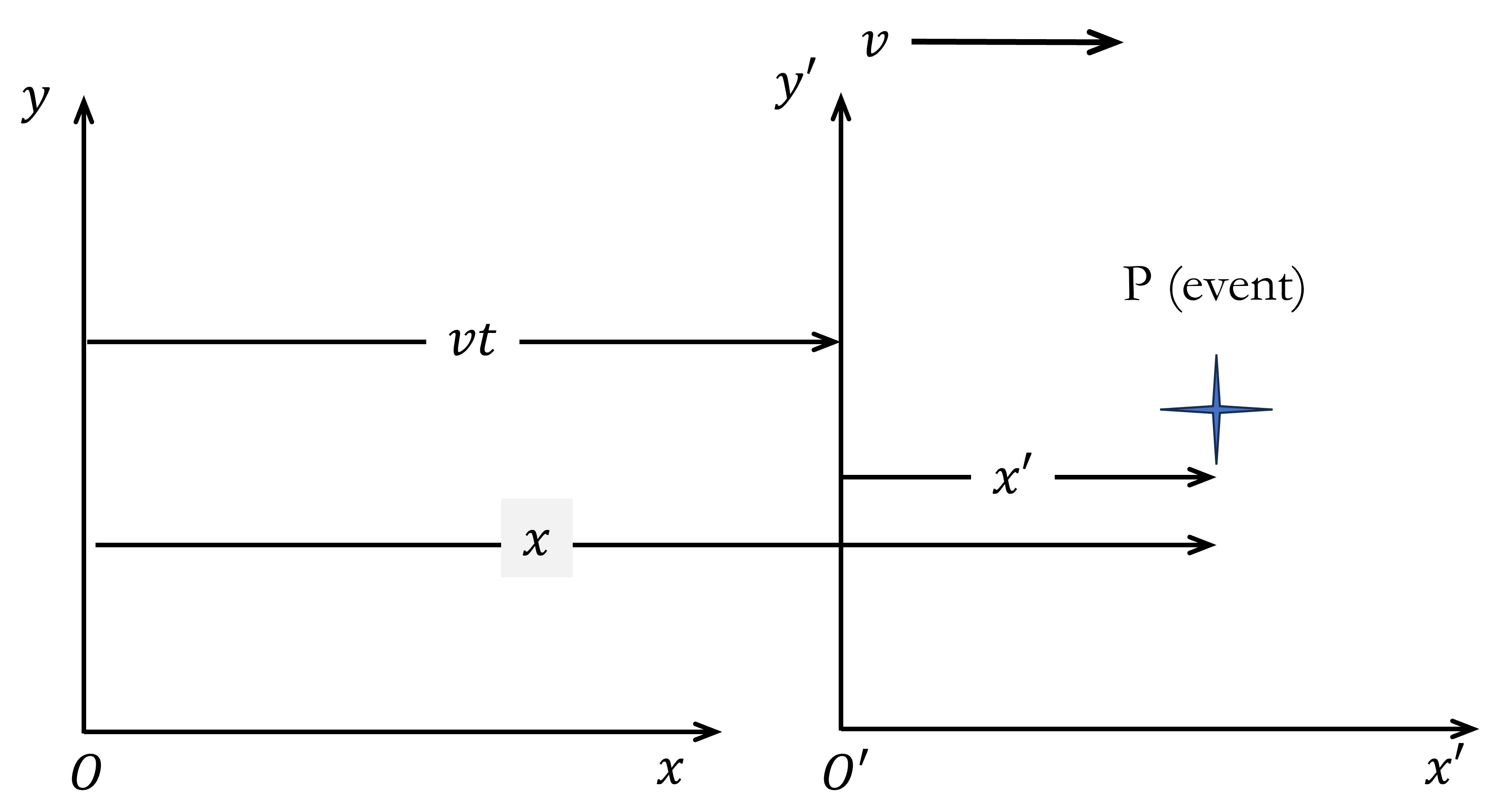
The event P can be described by frame S with space-time coordinates as ($x$, $y$, $z$, $t$), while in frame S’, it is described as ($x'$, $y'$, $z'$, $t'$). Now, let’s establish the relationship between space-time coordinates in the $S$ and $S'$frames, debited as:

\[\begin{eqnarray} x' &=& x -vt \tag{1.29} \\ y' &=& y \nonumber \\ z' &=& z \nonumber \\ t' &=& t \nonumber \end{eqnarray}\]

The above equations illustrate how to change the coordinate of an event from one frame to another when the two frames are moving at a constant speed in a straight line relative to each other. This transformation is known as the $\textbf{Galilean transformation of}$ $\textbf{coordinates}$ or simply the $\textbf{Galilean transformation}$. Here, we have made the assumtion that space and time are absolute and idependent of each other. This implies that the time of an event renaubs the same for all oversers, ragarless of their frame of reference. That’s why time varibale is consistent in both the $S$ and $S'$ frames ($t$ = $t'$). Here, where in classical mechanics all clocks run at the same rate regardless of their velocity. These assumption is incorrect when $v$ is comparable to the speed light.

Let’s consider the $\textbf{Inverse Galilean Transformation}$, in which the process of transforming coordinates from a moving frame of reference back to a stationary frame using the Galilean transformation.

\[\begin{eqnarray} x &=& x' + v t' \tag{1.30} \\ y &=& y' \nonumber \\ z &=& z' \nonumber\\ t &=& t' \nonumber \end{eqnarray}\]

Now, let’s explore the $\textbf{Galilean velocity transformations}$ by taking the derivative of position with resepect to time. The velocity transformations describe how the velocity of an object appears in two inertial frames of reference that are moving at a constant relative velocity with respect to each other. The transformation equation are outlined below:

\[\begin{eqnarray} u'_x &=& u_x -v \tag{1.31} \\ u_y' &=& u_y \nonumber\\ u_z' &=& u_z \nonumber \end{eqnarray}\]

Here, $u_x$ and $u'_x$ denote the instantaneous velocities of the object relative to the stantionary frame ($S$) and the moving frame ($S'$) respectively. Additionally, the change of time is the same in both frame, implying $dt$ = $dt'$.

Now, let’s explore the relationship between accelerations in $S$ and $S'$ frames. This can be obtained by taking derivative of velocity with respect to time.

\[\begin{eqnarray} a'_x &=& a_x \tag{1.32}\\ a'_y &=& a_y \nonumber\\ a'_z &=& a_z \nonumber \end{eqnarray}\]

The above equations indicate that the acceleration of an object is independent of inertial frame of reference, indicating the laws of physics are the same in all inertial frames. This constancy extends to length, time, mass, and accelerations, which are invariant under a Galilean transformation which are key concepts in classical mechanics. This consistency in acceleration is commonly referred to as the $\textbf{Equivalence Principle}$ in the context of inertial frames.

The Equivalence Principle holds additional significance, particularly in relation to gravity and relativity. It proposes that within a small region of space-time, the effects of gravity become indistinguishable from those of acceleration. Essentially, an observer in an accelerating room cannot discern the acceleration through local experiments, rendering the situation indistinguishable from being in a gravitational field. For example, dropping a ball in such a room results in it falling to the floor, irrespective of whether due to gravity or acceleration.

Originally proposed by Albert Einstein, the Equivalence Principle played a pivotal role in shaping the general theory of relativity. This transformative theory redefined our understanding of gravity, portraying it not as a force between masses but as the curvature of spacetime caused by mass and energy. Unlike classical mechanics, which assumes absolute and independent space and time, general relativity reveals their dynamic nature, subject to change based on the presence of mass and energy. This paradigm shift has profound implications for our comprehension of the fundamental nature of space, time, and gravitation.

Example 1.1. Roundtrip time in a stream

A swimmer is capable of swimming at a speed of $u$ in calm water. The swimmer is swimming in a stream with a current of $v$, where the speed of the current is less than the speed of the swimmer. Compare the time required to swim upstream for a distance $L$ and then returns downstream to the starting point with time needed to swim directly across the stream for a distance $L$ and back.

$\textbf{Solution}$

The swimmer always swim at speed $u$ relative to the water, and thus $u_x'= c$. According the Galilean transformation, speed of swimmer in earth frame when swimming upstream and downstream are \begin{eqnarray*} u_{x,u} &=& v - u \\ u_{x,d} &=& v + u \end{eqnarray*} where $u_{x,u}$ speed of swimmer respect to earth when swimming upstream and $u_{x,d}$ speed of swimmer respect to earth when swimming upstream. The total time to upstream and then return downstream to the strating point is \begin{eqnarray} t_{||} &=& \frac{L}{v-u}+ \frac{L}{v -u} \nonumber \\ t_{||} &=& \frac{2L}{u} \cdot \frac{1}{1-v^2/u^2} \tag{1.33} \end{eqnarray} Let's investigate where the swimmer swim directly across the stream. In this case, the velocity of the swimmer respect to earth frame need to be zero $u_x = 0 $. This requires, the swimmer needs to swim in the water frame with velocity $u_x' = -v $. Since the speed relative to the water is always $u $, we find that \begin{eqnarray*} u &=& \sqrt{u^2_{x'} + u^2_{y'}} \\ v_{y'} &=& \sqrt{u^2- v^2} \end{eqnarray*} So the round-trip time to swim directly across and back is \begin{eqnarray} t_{\perp} &=& \frac{2 L}{ \sqrt{u^2 -v^2}} = \frac{2L}{u} \cdot \frac{1}{\sqrt{1-\frac{v^2}{u^2}}} \tag{1.34} \label{eq:1-34} \end{eqnarray}

1.4 Conclusion

Classical physics is a powerful tool for describing the behavior of macroscopic objects accurately. However, its effectiveness is limited to specific scenarios such as speeds much lower than the speed of light, kinetic energies significantly below those associated with mass, and distances significantly exceeding atomic scales. As scientific exploration delved into the microscopic and high-speed domains, classical mechanics revealed its limitations, laying the foundation for the rise of modern physics. This transition marked a profound shift in our understanding of the universe. Modern physics, led by pioneering theories such as special relativity and quantum mechanics, has revolutionized our understanding of the universe.

eTextbooks, Computational-Aided Modern Physics

This post is licensed under CC BY 4.0 by the author.