Chapter 2: Special Relativity

Albert Einstein’s theory of special relativity revolutionized our understanding of the universe. This groundbreaking concept challenged and redefined our intuitive notions of space, time, and motion, initiating a new era in physics. Special relativity governs phenomena involving objects or reference frames moving at significant fractions of the speed of light, approximately \(3\times 10^8 \ m/s\), relative to one another.
Our everyday experiences occur at speeds far below this cosmic speed limit. Even spacecraft, which travel at impressive speeds around ~\(25,000\ mi/h (\approx 1.1 \times 10^4 m/s)\), only reach a tiny fraction of the speed of light. Because of our lack of direct experience with such high velocities, we often struggle to grasp the counterintuitive principles of special realtivity. However, through conceptual understanding and theoretical exploration, we can imagine a world where time and distance are not absolute, and where nothing can exceed the speed of light. This chapter will briefly introduce the concepts and theories of this revolutionary theory.

2.1 Introduction

Scottish physicist James Clerk Maxwell (1831-1879) made groundbreaking contributions to our understanding of electromagnetism. In the 1860s, he unified electricity, magnetism, and into a single theoretical framework. One of the remarkable implications through this unification was a theoretical prediction for the speed of light in a vacuum:

\[\begin{equation} c = \frac{1}{\sqrt{\mu_0 \epsilon_0}} \tag{2.1} \end{equation}\]

where c is the speed of light in a vacuum, \(\mu_0\) is permeability of free space (\(~ 4 \pi \times 10^{-7} N/A^2\) ) and \(\epsilon_0\) is permittivity of free space (\(~ = 8.854 \times 10^{-12} \ C^2/N.m^2\)).

In the 19^th, physicists believed that electromagnetic wave including light, required a medium for propagation like other waves. This hypothetical medium was called the “luminiferous ether,” thought to permeate all of space, including in vacuum. Particularly, the speed of light was assumed to be constant relative to this ether frame, leading scientist to believed that ether was delicate enought to allow celestial bodies such as planets to pass through it freely.

Albert A. Michelson (1952-1931) and American chemist Edward W. Morley (1838-1923).

Physicist assummed that the measurement of speed of light would change depending on the direction of light relative to the ether. To test the ether hypothesis, a rapidly moving frame was needed to detect any measurable change in the speed of light. In 1887, American physicists Albert A. Michelson and Edward W. Morley utilized the Earth’s motion aroung the sun \(\approx 30 \ km/s = 3 \times 10^4 m/s\). If the ether existed, it was hypothesized that the Earth’s motion through it would affect the measured speed of light in different directions.

To test this hypothesis, Michelson and Morley used a Michelson interferometer, a device that splits a beam of light into two perpendicular paths, reflects them off mirrors, and recombines them. Any difference in the speed of light in the two directions would result in an interference pattern. In the next section, we will delve deeper into the Michelson-Morley experiment and its implications for modern physics.

Schematic beam diagram of Mihelson-Morley experimental septup.

2.2 The Michelson-Morley Experiment

A Michelson interferometer, as depicted in Figure 2, was a crucial tool in the Michelson-Morley experiment. In this setup, a beam of light from a source is split by a beam splitter (M₀). One part of the split beam is reflected by mirror M₀, while the other part is reflected by mirror M₀. These reflected beams are then recombined at the beam splitter and reach the observer.

The interference of these two beams creates an interference pattern, form of a fringes pattern, typically observed as a series of dark and light fringes. This pattern is highly sensitive to any changes in the relative path lengths of the two beams.

To minimize external disturbances, the entire interferometer was mounted on a massive stone slab floating in a pool of mercury. This isolation technique reduced vibrations and temperature fluctuations, which could affect the interference pattern.

If the distance between M₀ and M₁ (Arm 2) is halved, the path length difference between the two beams changes. This results in a phase shift, causing the dark fringes to become bright and vice versa. This phenomenon is known as a fringe shift.

By carefully analyzing the interference pattern and any potential fringe shifts, Michelson and Morley aimed to detect the Earth’s motion through the hypothesized luminiferous ether.

The either wind direction respect to Arm 1 and Arm 2 can be change by rotate the entire instrument through 90\(^o\). It change could cause the fringe pattern to shift slightly.

Let’s recall Example 1.1 in the Chapter-1, where we analyzed the simplified scenario of swimmer swiming along the current and return. Using this example, we can show that the total time for the round-trip along along the horizontal path, considering the ether wind, is given by

\[\begin{eqnarray} t_1 &=& \frac{L}{c+v} + \frac{L}{c-v}= \frac{2 L c}{c^2-v^2} \nonumber \\ &=& \frac{2 L}{c} \left(1- \frac{v^2}{c^2} \right)^{-1} \tag{2.2} \end{eqnarray}\]

Similarly, recall the swiming across the river that we will get the light beam traveling perpendicular to the wind as

\[\begin{equation} t_2 = \frac{2 L}{\sqrt{c^2-v^2}} = \frac{2 L}{c} \left(1- \frac{v^2}{c^2}\right)^{-1/2} \tag{2.3} \end{equation}\]

From above two equations, the time difference between light beam traveling horizontally and vertically can written as:

\[\begin{equation} \Delta t = t_1 -t_2 = \frac{2 L}{c} \left[ \left(1- \frac{v^2}{c^2}\right)^{-1} - \left(1- \frac{v^2}{c^2}\right)^{-1/2} \right] \tag{2.4} \end{equation}\]

The time different, \(\Delta t\), represent the expected difference in the arrival times of the two light beams at the detector.

Since \(v^2/c^2 \ll 1\), we can use the binomial expansion to approximate the expressions, see Appendix Chapter 2. In our case, we can truncate the series after the second term, as higher-order terms are negligible.

In our case, \(x = v^2/c^2\), and we the time different between the light beam traveling horizontally and vertically is

\[\begin{equation} \Delta t = t_1 -t_2 \approx \frac{2L}{c} \left[ 1 + \frac{v^2}{c^2} -1 - \frac{v^2}{2 c^2}\right] = \frac{L v^2}{c^3} \tag{2.5} \end{equation}\]

Two light beams, initially in phase, interfere to produce a fringe pattern. A time difference between the beams, caused by the Earth’s motion, shifts the fringe pattern.

By rotating the interferometer 90 degrees horizontally, the roles of the two beams are exchanged. This doubles the path difference, resulting in:

\[\begin{eqnarray} \Delta d = c (2 \Delta t) = 2L \frac{v^2}{c^2} \tag{2.6} \end{eqnarray}\]

where \(\Delta d\) is the path difference, \(c\) is the speed of light, \(\Delta t\) is the time difference, \(L\) is the length of the interferometer arm, and \(v\) is the velocity of the Earth.

The fringe shift, assuming a linear relationship between path difference and fringe shift, is given by:

\[\begin{eqnarray} \text{Fringe Shift}=\left( \frac{2L}{\lambda} \right) \frac{ v^2}{c^2} \tag{2.7} \end{eqnarray}\]

where \(\lambda\) is the wavelenght of light.

The Michelson-Morley experiment was conducted at different times of the year to account for the Earth’s orbital motion. By rotating the interferometer, any potential differences in the speed of light in different directions could be detected.

Let’s calcualte the fringe shift: Typically Earth’s speed relative to the ether to 30 km/s, with a lenght L of 11 am, and using 500 nm light. We can expect the parth difference to be:

\[\begin{eqnarray*} \Delta d= \frac{2 (11m) (3 \times 10^4 m/s)^2}{3.0 \times 10^8 m/s)^2} = 2.2 \times 10^{-7} m \end{eqnarray*}\]

The fringe shift for a rotation through \(90^o\) is:

\[\begin{eqnarray*} \text{Fringe Shift}= \frac{\Delta d}{\lambda} = \frac{2.2 \times 10^{-7} m}{5.0 \times 10^{-7} m}\approx 0.40 \end{eqnarray*}\]

The Michelson-Morley experiment consistently failed to detect any significant fringe shift, despite the instrument’s ability to detect shifts as small as 0.1 fringes.

This null result contradicted the prevailing ether theory and led to a fundamental reassessment of the nature of light and space. It paved the way for Albert Einstein’s special theory of relativity, which introduced the concept of spacetime and the invariance of the speed of light in all inertial reference frame. Additionally, the Galilean transformations are not valid for inertial frames moving at high relative speeds. Albert Einstein addressed these issues in 1905 with his special theory of relativity

2.3 What is Special Relativity?

Newtonian mechanics is highly accurate for everyday activities, but it breaks down as the speed of a particle approaches the speed of light. Einstein’s Theory of Relativity is a more general framework, within which Newton’s laws of motion are a special case. Newton’s laws are valid approximations when the speeds of objects are much smaller than the speed of light (\(v \ll c\) ).

In 1905, at the age of 26, Albert Einstein published his special theory of relativity.

It is widely considered one of the greatest intellectual achievements in history.

Basic Postulates for Special Relativity:

The Principle of Relativity: The laws of physics are the same in all inertial reference frames. This means that the laws of physics take the same form for all observers moving at constant velocity relative to one another.

The Constancy of the Speed of Light: The speed of light is independent of the motion of the observer or the source of light, and the speed of light in a vacuum is always \(3 \times 10^8\) m/s.

Key Information:

• Relativity of Motion: There is no absolute motion; all motion is relative to a chosen reference frame.
• Ultimate Speed Limit: The speed of light represents the cosmic speed limit. No object with mass can reach or exceed this speed.
• Causality and Information Limit: Information cannot be transmitted faster than the speed of light, ensuring the principle of causality.

Medium Dependence: While the speed of light in a vacuum is constant, its speed in a medium (like water or glass) can vary. However, this variation is due to the properties of the medium itself, not the motion of the source or observer.

From Einsteen postulates, the following conclusion can be drown.

• 1^st postulate asserts that the laws of physics, encompassing electromagnetism, optics, thermodynamics, mechanics, and other fields, take the same form in all inertial reference frames.

• Limitation of Galilean Transformation: The Galilean transformation could not account for phenomena involving high velocities close to the speed of light. To address this limitation, Einstein adopted Lorentz transformations, which were originally developed by Hendrik Lorentz. These transformations correctly relate space and time between different inertial frames, ensuring that the form of physical laws remains invariant.

2.4 Time Dilation

Observers in different inertial reference frames always measure different time intervals. To derive this, let’s consider a classic example: a mirror is fixed to a moving vehicle. A light pulse is emitted from point O’, which is at rest relative to the vehicle.

For observer O’, the time taken for the light pulse to travel from O’ to the mirror and back again is:

\[\begin{eqnarray} \Delta t'= \frac{\mathrm{distance \ travel}}{speed\ of \ light} = \frac{2 d}{c} \tag{2.8} \end{eqnarray}\]

For observer (O), who is stationary relative to the vehicle, the light pulse must travel a longer diagonal path to hit the mirror and return to (O’).

According to the second postulate of special relativity, the speed of light is constant for all observers, regardless of their relative motion. Therefore, both observers must measure the speed of light as (c). Applying the Pythagorean theorem to the triangle formed by the light path, we get:

\(\begin{eqnarray*} \left(\frac{c \Delta t}{2}\right)^2 = \left(\frac{v \Delta t}{2}\right)^2 +d^2 \tag{2.9} \label{eq:2-9} \end{eqnarray*}\) Here, \(\Delta t\) is the time interval measured by observer (O), (v) is the velocity of the vehicle, and d is the distance between (O’) and the mirror in the vehicle’s frame. Solving for $\Delta t$ from eqaution \eqref{eq:2-9}, we get:

\[\begin{eqnarray} \Delta t = \frac{2 d}{\sqrt{c^2-v^2}} = \frac{2 d}{c \sqrt{1-v^2/c^2}} \tag{2.10} \end{eqnarray}\]

replacing 2d/c with ( \Delta t’ ), we can find that:

\[\begin{eqnarray} \Delta t= \frac{ \Delta t'}{ \sqrt{1-v^2/c^2}} = \gamma \Delta t' \tag{2.11} \label{eq:2-11} \end{eqnarray}\]

where:

• \(\gamma = \frac{1}{(1-v^2/c^2)}\) is the Lorentz factor. This factor represents the time dilation and length contraction experienced by an object moving at a relativistic speed.
• When \(v^2\) is positive (i.e., the object is moving), \(\gamma\) is greater than 1, indicating that the moving clock runs slower relative to a stationary clock.
• \(v^2 = \left(v_x^2 +v_y^2 +v_z^2\right)\).

We can see that \(\Delta t\) is greater than \(\Delta t\). This result indicates that the time interval \(\Delta t\), measured by the stationary observer, is longer than the time interval \(\Delta t'\), measured by the observed mocing with the clock. This effect is known as time dilation.

Typically, \(\Delta t'\) is referred to as the proper time ($\Delta t_p$). In general, we can rewrite as \ref{eq:2-11}:

\[\begin{eqnarray} \Delta t = \gamma \Delta t_p \tag{2.12} \end{eqnarray}\]

We can also say that:

A moving clock runs slower than a clock at rest by a factor of \(\gamma\).

Time dilation affects all physical processes, including chemical reactions and biological processes. Here, all physical processes slow down when observed from a reference frame in which they are moving. It is a very real phenomenon that has been verified by various experiments, such as the Hafele-Keating experiment, where atomic clocks were flown around the world on commercial airliners

Example 1.1. Muon Mystery: How Do They Reach Earth?

Muons are unstable elementary particles with a charge equal to that of an (\(e\)) and a mass approximately 207 times that of an electron. Muons are primarily produced from the decay of pions (\(\pi^+\) or (\(\pi^-\)), which are generated when high-energy cosmic rays collide with atoms in the Earth's atmosphere.
Although muons have a relatively short half-life (\(2.2 \mu s\)), many of them reach the Earth's surface due to relativistic time dilation. This phenomenon, predicted by Einstein's theory of relativity, slows down the decay of muons from our perspective on Earth.
Muon production due to pions, The production of muons through pion decay follows the reactions: $$\begin{eqnarray*} \pi^+ &\rightarrow&  \mu^+ +\nu_\mu \\ \pi^- &\rightarrow& \mu^- +\overline{\nu}_\mu \end{eqnarray*}$$ Here,\(\pi^+\) and \(\pi^-\) are charged pions, \(mu^+\) and \(\mu^-\) are positively and negatively charged muons, \(\nu_\mu\) is the muon neutrino, and \(\overline{\nu}_\mu\) is the muon antineutrino. The muon is a lepton that decays into an electron or positron and two neutrinos: $$\begin{eqnarray*} \mu^- \rightarrow e^- +\overline{\nu}_e +\nu_\mu \nonumber \\ \mu^+ \rightarrow e^+ +\nu_e +\overline{\nu}_\mu \nonumber \end{eqnarray*}$$ In each decay, a muon decays into an electron or positron, an electron antineutrino (\(\overline{\nu}_e \)) or electron neutrino (\( \nu_e \)), and a muon antineutrino ( \(\overline{\nu}_\mu\)) or muon neutrino ((\nu_\mu\)).
Muons have a rest lifetime of 2.2 \(\mu s\) (proper time). Traveling near the speed of light, a muon could typically travel about 650 m before decaying. At this rate, they wouldn't reach the Earth's surface from their point of origin in the upper atmosphere.
However, experiments have shown that a significant number of muons do reach the Earth's surface. This discrepancy is explained by the phenomenon of time dilation.
We can estimate the apparent time dilation experienced by muons in the Earth's frame of reference:
If the speed of the muons is approximately 0.99c, then: $$\begin{eqnarray*} \gamma = \frac{1}{\sqrt{1-v^2/c^2}} \approx 7.1 \Rightarrow \gamma \tau \approx 16 \mu s \end{eqnarray*}$$ The average distance traveled as measured by an observer on Earth is $$\begin{eqnarray*} v (\gamma \tau) \approx 4700 m \end{eqnarray*}$$ This muon time dilation was experiment investiate. In 1976, experiments at CERN involved accelerating muons to speeds of 0.9994 times the speed of light. It was observed that the lifetime of these high-speed muons was approximately 30 times longer than that of stationary muons. This experimental result provides strong evidence for the theory of special relativity and the concept of time dilation.

Another actual experimental evidence for time dilation comes from the Hafele-Keating experiment, where cesium atomic clocks were flown around the world on commercial airliners. The clocks on the planes were observed to run slightly slower than identical clocks that remained on the ground, confirming the prediction of time dilation. This experiment provided strong experimental evidence supporting the theory of special relativity.

Example 1.2. Pendulum in moving frame

A pendulum has a period of 4 seconds in its rest frame. What is its period as measured by an observer moving at 0.85c relative to the pendulum?

2.4.1 The Twin Paradox

The twin paradox is a classic thought experiment in special relativity. It involves two twins, one who stays on Earth while the other travels at a significant fraction of the speed of light on a round trip journey. Upon returning, the traveling twin is found to be younger than the stay-at-home twin.

As Einstein originally stated in 1911:

If we place a living organism in a box… one could arrange that the organism, after an arbitrary lengthy flight, could be returned to its original spot in a scarcely altered condition, while corresponding organisms which had remained in their original positions had long since given way to new generations.

2.5 Length Contraction

Similar to time, the distance between two points also depends on the frame of reference in which it is measured. The length of an object measured in its rest frame is called its proper length.

When an object moves relative to an observer, its length appears to be contracted in the direction of motion. This phenomenon is known as length contraction.

Let’s estimate the lenght conctraction through drivation. Consider a rod of length \(L\) at rest in frame S’. An observer in frame S, moving with a velocity \(u\) relative to S’, measures the length of the rod.

To measure the length of the rod, the observer in S sends a light signal from point A to point B and back, timing the round trip. The light travels a distance \(L + u \Delta t_1\) to reach point B and a distance \(L - u \Delta t_2\) to return to point A.

The time taken for the dround trip is:

\[\begin{equation} \Delta = \Delta t_1 + \Delta t_2 \tag{2.13} \end{equation}\]

Using the speed of light, c:

\[\begin{eqnarray*} c \Delta t_1 &=& L + u \Delta t_1 \\ c \Delta t_2 &=& L - u \Delta t_2 \end{eqnarray*}\]

Adding these equations, we find the total time:

\[\begin{eqnarray} \Delta t &=& \Delta t_1 + \Delta t_2 = \frac{L}{c-u} + \frac{L}{c+u} \nonumber \\ &=& \frac{2L}{c} \frac{1}{\left(1- u^2/c^2 \right)} \tag{2.14} \label{eq:2-14} \end{eqnarray}\]

From the time dilation formula:

\[\begin{eqnarray} \Delta t &=& \gamma \Delta t_p= \frac{\Delta t_p} {\sqrt{1- u^2/c^2}} \nonumber \\ &=& \frac{2 L_p}{c} \frac{1} {\sqrt{1- u^2/c^2}} \tag{2.15} \label{eq:2-15} \end{eqnarray}\]

from above two equations \ref{eq:2-14} and (\ref{eq:2-15}):

\[\begin{eqnarray*} L &=& L_p \sqrt{1- u^2/c^2} \Rightarrow L = \frac{L_p}{\gamma} \tag{2.16} \label{eq:2-16} \end{eqnarray*}\]

This equation shows that the length \(L\) measured by an observer in a moving frame is shorter than the proper length \(L_p\) of the object at rest. This phenomenon is known as length contraction.

As shown in the figure, the length of an object contracts in the direction of motion as its speed approaches the speed of light.

2.6 Clock Synchorization

In the framework of special relativity, the concepts of distance and time are not absolute but are relative to the observer’s frame of reference. This means that the spatial separation between two points and the time interval between two events can vary depending on the relative motion of the observer.

To accurately measure distances and time intervals in different reference frames, it’s crucial to synchronize clocks. This synchronization process relies on the principle that the speed of light is constant in all inertial reference frames, regardless of the observer’s motion or the light source’s motion.

The synchronization process involves sending a light signal between two points and assuming that the light travels at the same speed in all directions. By measuring the time it takes for the light signal to travel and return, observers can define a common time across their reference frame.This method ensures consistency in measurements of time and space, allowing for meaningful comparisons between events observed in different inertial frames.

Relativity of Simultaneity: One of the most counterintuitive consequences of special relativity is the relativity of simultaneity. Two events that are simultaneous in one inertial frame may not be simultaneous in another inertial frame moving relative to the first.

This means that the concept of simultaneity is not absolute but depends on the observer’s frame of reference.

Example 1.3. Syncrhorization Correction

For instance, consider a train moving at a significant fraction of the speed of light. If lightning strikes the front and back of the train simultaneously according to an observer standing on the platform, a passenger on the train will perceive the lightning strike the front of the train first. This discrepancy arises from the finite speed of light and the relative motion between the observer and the train.
The difference in the perceived timing of the events arises from the finite speed of light and the relative motion of the observers. This phenomenon is known as the relativity of simultaneity.
Derivation of Syncrhonization Correction Term
To quantify this time difference, we calculate the synchronization correction term, \(\tau_s \), which represents the time discrepancy observed in the two frames. Consider the following:

1. Let the train car have a length \(\Delta x\) in the rest frame \(S\).
2. Let the front strike light reach center at \(t_A\) and the back strike reach center at \(t_B\) as observed in \(S\).

Using the principle of constant light speed and accounting for the relative motion of the train, the time taken for light to reach the midpoint of the train car is:
$$\begin{eqnarray*} \frac{1}{2} \Delta x &=& (c +v) t_A \ \Rightarrow t_A = \frac{1}{2} \frac{\Delta x}{c+v} \end{eqnarray*}$$ and similarly, $$\begin{eqnarray*} \frac{1}{2} \Delta x &=& (c-v) t_B \ \Rightarrow t_B = \frac{1}{2} \frac{\Delta x}{c-v} \end{eqnarray*}$$ The synchronization correction term $\tau_s$ is: $$\begin{equation*} \tau_s = t_B - t_A = \frac{1}{2} \Delta x \left( \frac{1}{c-v} - \frac{1}{c+v}\right) \end{equation*}$$ Simplifying: $$\begin{eqnarray*} \tau_s &=& \frac{\Delta x}{\left( 1- \frac{v^2}{c^2}\right)} \frac{v}{c^2} \end{eqnarray*}$$ Using the Lorentz factor \(\gamma = 1/\sqrt{1-v^2/c^2}\), we rewrite: $$\begin{eqnarray*} \tau_s = \gamma \frac{\Delta x' v}{c^2} \end{eqnarray*}$$ where \( \Delta x' = \gamma \Delta x \) The synchronization correction term \(\tau_s\) : $$ \begin{equation*} \tau_s = \gamma \frac{\Delta x_p v}{c^2} \tag{2.17} \end{equation*}$$ It differs fundamentally from the previously discussed time dilation effect. While time dilation concerns the slowing of clocks due to relative motion, \(\tau_s\) reflects the perceived timing discrepancy of events due to relative motion and the finite speed of light.
For convenience, we isolate the time dilation effect by expressing: \begin{equation*} \tau_s = \gamma \tau'_s \end{equation*} where: \begin{equation*} \tau'_s = \frac{\Delta x_p u}{c^2} \end{equation*} is the time discrepancy as calculated by observers in \(𝑆\) for events in \(S'\). This form makes it clear that \(\tau'_s\) must be interpreted as the time discrepancy expected by observes in \(S\) to exist between the clocks in \(S'\).

The relativity of simultaneity reveals how the perception of events occurring simultaneously depends on the observer’s frame of reference. Events that appear simultaneous in one frame may not be simultaneous in another. This concept underscores the intricate relationship between time and space, highlighting their interconnectedness within the fabric of spacetime.

The relativity of simultaneity challenges our intuitive understanding of time and space, leading to profound implications for our perception of the universe. It demonstrates that time and space are not absolute but rather relative to the observer’s motion, paving the way for a deeper understanding of the nature of reality.

2.5 Doppler Effect

We have learned that observed frequency of a sound waves depend on the relative speed of the source and the observer, which was first suggest by Christine Johann Doppler (1803-1853}. These shift frequency of sounds is called (classical) Doppler effect. The observed frequency of wave depend on the relative speed of source and observer, and it can be expresses as:

\(\begin{eqnarray} f_o = f_s \left(\frac{v\pm v_0}{v\mp v_s} \right) \tag{2.18} \label{eq:2-18} \end{eqnarray}\) where:

• \(f_o\) is the frequency heard by the observer,
• \(f_s\) is the frequency of source,
• \(v\) is the speed of the waves in the medium,
• \(v_s\) is the speed of source relative to medium,
• \(v_o\) is the speed of observer relative to the medium.

In the \ref{eq:2-18}, the upper signs of numerator and denominator are chosen whenever observer moves toward or away from source determine the upper sign, while lower signs apply whenever source moves toward or away from observer.

Similar to effect of frequency of sound due to frame motion, the frequency of light have varies too. If an frame speed reach close to speed of light, due to consequence of time dilation, the frequency of light is founded to shift. Here, light wave must be analyzed differently from sound, because light require no medium of propagation and speed of light independent of frame.

Lets consider a source light at rest frame S (Figure), and emitting waves of frequency f and wavelength \(\lambda\). We need to find frequency \(f'\) and wavelength \(\lambda'\).

We know by observation (in general) that \(f'\) is greater than \(f\) when \(S'\) approach because more wave crests are crossed per unit time. Similarly, we can expect \(f'\) is less than \(f\) is \(S'\) recedes from S.

Let’s look at the two successive wave-fronts positions 1 and 2 of light wave when approaching source, see the Figure. The wavelength can be written as:

\[\begin{equation*} c = f \lambda = \frac{1}{T} \lambda \Rightarrow \lambda = c T \end{equation*}\]

The successive wave-fronts (wavelength) will be measured in observer frame S’ to be

\[\begin{eqnarray} \lambda' = c T'- v T' \tag{2.19} \end{eqnarray}\]

The frequency can be written as

\[\begin{eqnarray} f' = \frac{c}{\lambda'} = \frac{c}{(c- v) T'} \Rightarrow \frac{1}{T'} = \frac{(c-v)}{c} f' \tag{2.20} \end{eqnarray}\]

From time dilation expression, we get:

\[\begin{eqnarray*} T ' = \gamma T \\ \Rightarrow \frac{1}{T'} =\sqrt{(1-v^2/c^2)} \frac{1} {T} \end{eqnarray*}\]

by substituting \(1/T = f\) and \(1/T' = (c-v) f'/c\), we get:

\[\begin{eqnarray*} f' &=& \frac{\sqrt{1- v^2/c^2}}{(1-v/c)} f \end{eqnarray*}\]

It can be also rewritten as:

\[\begin{equation*} f'= \frac{\sqrt{1+v/c}}{\sqrt{1- v/c}} f \end{equation*}\]

we can rewrite as \(\begin{eqnarray} f_o &=& \frac{\sqrt{1+ v/c}}{\sqrt{1- v/c}} f_s \\ f_o &=& \frac{\sqrt{1+ \beta}}{\sqrt{1- \beta}} f_s \tag{2.21} \end{eqnarray}\)

where \(\beta = v/c\), \(f_o\) is frequency of light observed, and \(f_s\) is source frequency of light.

Unlike the Doppler formula for sound, depends only on the relative speed \(v\) of the source and observer. \(f_{obs}\) to be greater than \(f_{source}\)

The most spectacular and dramatic use of the Doppler effect has observed in red shift absorption lines for most galaxies. This suggest that galaxies are rapidly receding from us.

2.6 Lorentz Transformation

Galilean transformations, which were fomulated for the Newtonian mechanics, describe the relationships between space and time coordinates in different reference frames. However, they break down when dealing with objects moving at speeds approaching the speed of light. To address this limitation, we need a new set of transformations, Lorentz Transformations. The Lorentz transformations were developed by the Dutch physicist Hendrik A. Lorentz (1853-1928) and are fundamental to the theory of special relativity.

2.6.1 Space and Time

First, we will derive the Lorentz transformations equations, which accurately describe the relationships between space and time coordinates in different inertial reference frames moving at relativistic speeds, close speed of light.

Let’s consider an inertial reference frame \(S'(x',y',z',t')\) moving in the x-direction with a speed of \(v\)/4 relative to another inertial reference frame \(S(x,y,z,t)\). The relationship between these two frames using Galilean transformations is given by:

\[\begin{eqnarray} x' &=& x - vt \nonumber \\ y' &=& y \nonumber \\ z' &=& z \nonumber\\ t' &=& t \tag{2.22} \end{eqnarray}\]

When the frame approach speed of light, we consider that distance is change by a dimensionless factor \(g\). Now the new position can be written as:

\[\begin{eqnarray} x' &=& g(x- vt) \nonumber \\ y' &=& y \nonumber \\ z' &=& z \tag{2.23} \label{eq:2-23} \end{eqnarray}\]

One can note that it forms the Galilean transformation when \(G = 1\).

If \ref{eq:2-23} is correct, the inverse transformation should correct and it can be written as:

\[\begin{eqnarray} x &= & g(x' + vt') \nonumber \\ y &=& y' \nonumber \\ z &=& z' \tag{2.24} \label{eq:2-24} \end{eqnarray}\]

Replacing \(x'\) in equation \ref{eq:2-24} from eqaution \ref{eq:2-23} gives:

\[\begin{eqnarray} x &=& g \left( g (x- vt ) + v t'\right) \nonumber \\ \end{eqnarray}\]

and simplification yields to: \(\begin{eqnarray} t' &=& g \left[t + \left(1/g^2 -1\right) \frac{x}{v}\right] \tag{2.25} \label{eq:2-25} \end{eqnarray}\)

The differential of equations \ref{eq:2-23}, yields to:

\[\begin{eqnarray} dx' = g(dx- v dt) \tag{2.26} \label{eq:2-26} \end{eqnarray}\]

The differential of equations \ref{eq:2-25}, yields to:

\[\begin{eqnarray} dt' &=& g \left[dt + \left(1/g^2 -1\right) \frac{dx}{v}\right] \tag{2.27} \label{eq:2-27} \end{eqnarray}\]

Through recalling \(u'_x = dx'/dt'\) and \(u_x = dx/dt\), combining equations \ref{eq:2-26} and \ref{eq:2-27}, gives:

\[\begin{eqnarray} u_{x'}= \frac{u_x -v}{1+ (1/g^2 -1)(u_x/v))} \tag{2.28} \label{eq:2-28} \end{eqnarray}\]

Above eqaution should satisfy for photon frame (frame moving with speed of light). From postulate 2 of special realativity that speed of light to be constant \(c\) for any observer. In this case \(u_x = c\) and \(u_x' = c\). \ref{eq:2-28} reduces to:

\[\begin{eqnarray*} c &=& \frac{c -v}{1+ \left(1/g^2 -1\right) (c/v)} \end{eqnarray*}\]

Simplication yeilds to:

\[\begin{eqnarray} g = \frac{1}{\sqrt{1- (v^2/c^2)}} = \gamma \end{eqnarray}\]

By substituting g with \(\gamma\):

\[\begin{eqnarray} x' &=& \gamma (x - vt) \nonumber \\ y' &=& y \nonumber \\ z' &=& z \nonumber \\ t' &=& \gamma \left(t- \frac{v x}{c^2}\right) \tag{2.29} \end{eqnarray}\]

Above equations are called Lorentz transformation of \(S \rightarrow S'\) and the inverse transformation by simply replace \(v\) by \(-v\) and gives

\[\begin{eqnarray} x &=& \gamma ( x'+ vt) \nonumber \\ y &=& y' \nonumber \\ z &=& z' \nonumber \\ t &=& \gamma \left( t' + \frac{v x'}{c^2}\right) \tag{2.30} \end{eqnarray}\]

Note that when \(v/c <1\) and \(v^2/c^2 \ll 1\), it reduce to Galilean coordinate transformation, given by.

2.6.2 Velocities

From eqaution \ref{eq:2-28} we find immediately by substituting \(g = \gamma = 1/\sqrt{1-(v^2/c^2)}\)

\[\begin{eqnarray} u'_x = \frac{u_x -v}{1- \left( u_x v / c^2 \right)} \tag{2.31} \end{eqnarray}\]

We can find he velocity component along y and z in \(S'\)

\[\begin{eqnarray} u'_y &=& \frac{dy'}{dt'}= \frac{u_y}{\gamma \left(1 - v u_x /c^2\right)} \\ u'_z &=& \frac{u_z}{\gamma \left(1 - v u_x /c^2\right)} \tag{2.32} \end{eqnarray}\]

When \(u_x\) and v are both much smaller than c, non-relativistic case, we see \(u'_x \approx u_x - v\). This corresponding to the Galilean velocity transformation.

In other extreme, when \(u_x =c\)

\[\begin{equation*} u'_x = \frac{c -v}{1 - (c v / c^2)} = c \end{equation*}\]

From above, we see that an object moving with a speed c relative to observer S and observer S’ -\textit{independent} of the relative motion of S and \(S'\). This agree with Einstein’s 2nd postulate that speed of light must be c in all frame and speed of an object never exceed c.

Inverse Transformation is

\[\begin{eqnarray} u_x &=& \frac{u_{x'} + v}{1+ (u_{x'} v/c^2)} \nonumber \\ u_y &=& \frac{u_y'}{\gamma \left(1 + v u_x' /c^2\right)} \\ & \text{and} \nonumber \\ u_z &=& \frac{u_z'}{\gamma \left(1 - v u_x' /c^2\right)} \tag{2.33} \end{eqnarray}\]

2.7 Minkowski Space-Time Diagram

German mathematician Hermann Minkowski recognized that Einstein’s theory of special relativity could be elegantly interpreted within the framework of a four-dimensional spacetime, where time is treated as a dimension alongside the three spatial dimensions. In 1908, Minkowski developed the spacetime diagram, a graphical representation that provides a powerful visual understanding of the phenomena of time dilation and length contraction without relying on complex mathematical equations.

Schematic diagram of spacetime diagram that shows the world line of particle and particle at rest.

The spacetime diagram is similar to the position-versus-time graphs used in introductory physics, but with a significant difference: time is plotted on the vertical axis and space on the horizontal axis. This allows for a more intuitive representation of relativistic effects, including the twin paradox.

In this course, we will use a two-dimensional spacetime diagram to simplify visualization (Figure).

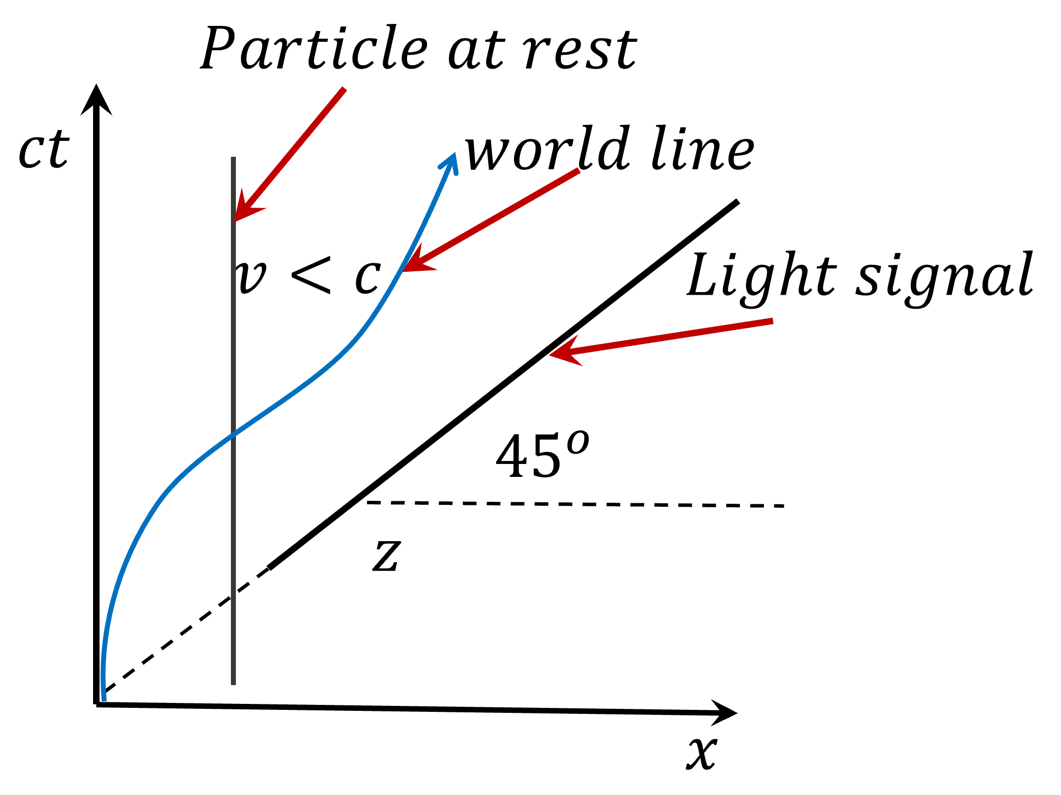
In a spacetime diagram, a moving particle traces out a line called its worldline.

• In a traditional position vs. time graph, the velocity of a particle is determined by finding the slope of the line.
• In spacetime diagram, the inverse slope of the worldline gives the particle’s velocity. The exact relationship depends on the speed of light.
• A vertical line represents a particle that is at the same spatial location at all times—that is, a particle at rest.

\[\begin{eqnarray} \text{slop} &=& \frac{\Delta (ct)}{\Delta x} = \frac{c}{v} \nonumber \\ v &=& \frac{c}{\text{slop}} \tag{2.34} \end{eqnarray}\]

The Figure shows a spacetime diagram drawn in the laboratory frame. Here, the speed of light is represented by a line with a slope of 1 (\(45^o\) degree) in units where the time and space axes have the same scale (often referred to as “lightcone”). Permitted motions with constant velocity are then represented by straight lines within the lightcone.

Minkowski diagrams can be used to classify the entire universe of spacetime and clarify whether or not one event could causally influence another.

• The regions labeled “past” and “future” correspond to events that could be causally connected to the event at the origin (the “present”).
• The region labeled “elsewhere” represents events that cannot be causally connected to the event at the origin. To reach these events would require traveling faster than the speed of light, which is physically impossible according to the theory of relativity.

In the new frame, the spacetime coordinates are denoted as x’ and ct’. Similarly, we can draw a new spacetime diagram and plot the worldline using these new coordinates.

Crucially, x’ and ct’ must be constructed in such a way that the speed of light remains constant in all inertial frames. This is a fundamental postulate of special relativity. We can see (Figure) that in inertial frames (S’), the ct’ and x’ axes are not orthogonal, unlike in the usual Cartesian coordinate system

Here, both systems are coincide at \(t = t' =0\) and \(x = 0 =x'\). Let’s apply Lorentz transformation:

\[\begin{equation*} x' = \gamma (x - vt) = 0 \ \ \text{for } \ \ x' =0 \end{equation*}\]

it gives

\[\begin{equation*} ct = \left(\frac{1}{\beta}\right) x \ \Rightarrow \ \ \frac{ct}{v} = \frac{1}{\beta} \end{equation*}\]

The slop observed in S frame of the worldline of the point \(x'=0\), the \(ct'\). Similarly, we can apply Lorentz transformation once again for time that gives the slop:

\[\begin{eqnarray*} t ' &=& \gamma( t - \frac{v x}{c^2}) = 0 \\ \frac{ct}{v} &=& \frac{1}{\beta} \end{eqnarray*}\]

Slop of the \(x'\) axis as measured by an observed is S is \(\beta = ct/x = v /c\). Note that x -axes don’t parallel anymore. Actually, they are still parallel in space, but this is a spacetime diagram.

Let’s consider two events happen (\(E_1\) and \(E_2\)). In the S frame, we can write that

\[\begin{eqnarray*} (\Delta s)^2 &=& - \left((\Delta x)^2 + (i c \Delta t)^2 \right) \\ (\Delta s)^2 &=& (c \Delta t)^2 -(\Delta x)^2 = (c(t_2-t_1))^2 - (x_2-x_1)^2 \end{eqnarray*}\]

Similarly, in \(S'\) frame

\[\begin{eqnarray*} (c \Delta t')^2 -(\Delta x')^2 = (c(t'_2-t'_1))^2 - (x'_2-x'_1)^2 \end{eqnarray*}\]

\(S'\) and \(S\) frames are connected by the Lorentz transforms

\[\begin{eqnarray*} x'_1 &=& \gamma (x_1- v t_1) \\ t'_1 &=& \gamma (t_1 - v x_1/c^2) \end{eqnarray*}\]

we find that:

\[\begin{eqnarray*} (\Delta s')^2 &=& \gamma^2 \left[ c^2 \left( (t_2 - v x_2/c^2) - (t_1 - v x_1/c^2)\right)^2 -\left((x_2- v t_2) - (x_1- v t_1)\right)^2 \right] \\ &=& \gamma^2 \left[ c^2 \left( (t_2 - t_1)- \frac{v}{c^2}(x_2- x_1)\right)^2 -\left((x_2-x_1) - v(t_2- t_1)\right)^2 \right] \\ &=& \gamma^2 \left[(t_2 - t_1)^2 (c^2 -v^2)+ (x_2- x_1)^2 \left(\frac{v^2}{c^2}- 1\right) \right] \\ &=& \gamma^2 \left[c^2(t_2 - t_1)^2 - (x_2- x_1)^2 \right] \left(1- \frac{v^2}{c^2}\right)= (c \Delta t)^2 - (\Delta x)^2\\ &=& (\Delta s)^2 \end{eqnarray*}\]

This result demonstrates that the spacetime interval, denoted by \((\Delta s)\), between two events is an invariant quantity. This means that \((\Delta s)\) has the same value for all inertial observers, regardless of their relative motion