Chapter 4: States of a Model System
This chapter describe the binary system.
4.1 Introduction
Both thermodynamics and statistical mechanics describe the behavior of physical systems that contain an enormous number of degrees of freedom. A macroscopic system typically consists of an immense number of microscopic constituents—atoms or molecules—each of which can exist in many possible states. Consequently, such systems possess a huge number of possible microscopic configurations.
In classical Newtonian mechanics or quantum mechanics, physical systems are usually analyzed by applying fundamental dynamical laws together with conservation principles such as conservation of energy, momentum, and angular momentum. These approaches work very well when dealing with systems containing only a few degrees of freedom. However, when the number of particles becomes extremely large—on the order of Avogadro’s number (\(10^{23}\) particles in one mole of gas)—the direct application of Newton’s equations or the Schrödinger equation becomes practically impossible.
Fortunately, nature provides a powerful quantity that allows us to deal with this enormous complexity: entropy. Entropy serves as a measure of the number of ways in which a system can be arranged microscopically while still producing the same macroscopic behavior. Thermodynamics shows that entropy, together with conservation laws, forms one of the fundamental building blocks for describing the macroscopic properties of complex systems.
This raises an important question: Is complete knowledge of the fundamental laws of nature sufficient to understand the macroscopic world around us? Suppose we knew all the properties of elementary particles, their masses, charges, and the forces governing their interactions, as well as the equations describing their dynamics. In principle, such knowledge should allow us to determine the behavior of any physical system. However, in practice, solving the equations of motion for systems containing an enormous number of interacting particles is computationally impossible.
For example, consider a gas containing one mole of molecules. Even if we know all the interactions between these molecules, solving the full set of Newtonian or quantum mechanical equations for approximately 1023 particles is far beyond our capabilities. Instead, we require a different approach—one that does not attempt to track every particle individually. This approach is statistical mechanics.
Statistical mechanics provides a framework for understanding the macroscopic properties of matter by studying the statistical behavior of large collections of particles. By focusing on probabilities and averages rather than exact microscopic details, statistical mechanics allows us to connect microscopic physical laws with macroscopic thermodynamic quantities such as temperature, pressure, and energy.
Because of this broad applicability, statistical mechanics plays a central role in many areas of physics, including astrophysics, condensed matter physics, atomic physics, and nuclear physics. It is often regarded as a theory of remarkable elegance because it provides a simple conceptual framework for describing systems of enormous complexity.
Microstates and Macrostates
A microstate of a multiparticle system is a complete specification of the states of all the particles in the system. For a system containing N particles, a microstate is defined when the individual states of all 𝑁 particles are known.
In practice, however, we usually know only a limited set of macroscopic variables, such as temperature, pressure, volume, density, and total energy. Such a description corresponds to a macrostate.
Many different microstates can correspond to the same macrostate. Statistical mechanics studies how the number and distribution of these microstates determine the observable thermodynamic properties of the system.
Goal of Statistical Mechanics : Starting from the possible microstates of a system and their associated multiplicities (degeneracies), we aim to determine the macroscopic thermodynamic properties of the system.
In this way, statistical mechanics provides the essential bridge between microscopic physical laws and macroscopic thermodynamic behavior.
4.3 Binary Model System
We begin our discussion with a simple binary model system, in which each of the N particles (or sites) that constitute the system can occupy one of two possible single-particle states. Despite its simplicity, this model captures many essential ideas of statistical mechanics and provides a useful framework for understanding more complex systems.
Consider a set of N distinct and fixed sites arranged, for example, along a one-dimensional lattice. Because these sites are fixed in space, they are distinguishable from one another. For instance, the first site from the left can be distinguished from the fifth site from the right. Each site therefore represents a unique location in the system.
At each site there exists a property that can take only two possible values. Consequently, each site has two allowed states, and the entire system can be described by specifying the state of every site.
A useful physical example of such a system is a one-dimensional array of N non-interacting spins, where each spin can point either up or down. These two orientations represent the two possible states of each site.
This simple model will allow us to explore important concepts such as microstates, multiplicity, and entropy, which are fundamental to the statistical description of macroscopic systems.
Let us consider a simple example of a \textbf{binary spin system} with $N = 3$ spins. Each spin can exist in two possible states: \textit{up} $(\uparrow)$ or \textit{down} $(\downarrow)$.
For \textbf{spin 1}, there are two possible states: up or down.
For each state of spin 1, spin 2 can also take two possible states. Therefore the pair \((\text{spin 1}, \text{spin 2})\) has
possible configurations.
For each configuration of spins 1 and 2, spin 3 again has two possible states. Thus the total number of configurations for a system of three spins is
\[2 \times 2 \times 2 = 2^3 = 8\]These configurations represent the \textbf{microstates} of the system.
Microstates for N=3
| Description | Spins | Possibilities | Spin Excess |
|---|---|---|---|
| All three up | ↑↑↑ | 1 | Up−down = 3−0 = 3 |
| Two up and one down | ↑↑↓, ↑↓↑, ↓↑↑ | 3 | Up−down = 2−1 = 1 |
| One up and two down | ↑↓↓, ↓↑↓, ↓↓↑ | 3 | Up−down = 1−2 = −1 |
| All three down | ↓↓↓ | 1 | Up−down = 0−3 = −3 |
For a system with $N = 3$ spins, we found that there are 8 possible microstates
\[8 = 2^3 = 2^N\]In addition, the number of possible values of the spin excess (or magnetization) is
\[4 = 3 + 1 = N + 1\]Let us now consider a system of N = 4 spins.
| Description | Spins | Possibilities | Spin Excess |
|---|---|---|---|
| All four up | ↑↑↑↑ | 1 | Up − down = 4-0=4 |
| Three up and one down | ↑↑↑↓, ↑↑↓↑, ↑↓↑↑, ↓↑↑↑ | 4 | Up − down = 3-1=2 |
| Two up and two down | ↑↑↓↓, ↑↓↑↓, ↓↑↑↓, ↑↓↓↑, ↓↑↓↑, ↓↓↑↑ | 6 | Up − down = 2-2=0 |
| One up and three down | ↑↓↓↓, ↓↑↓↓, ↓↓↑↓, ↓↓↓↑ | 4 | Up − down = 1-3=-2 |
| All four down | ↓↓↓↓ | 1 | Up − down = 0-4=-4 |
Thus, there are 16 different microstates and five different values of the spin excess (or magnetization).
Since N = 4 in this case, we can write
\[2^4 = 16 = 2^N\]microstates, and
\[4 + 1 = 5 = N + 1\]possible values of the magnetization.
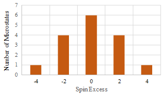
Figure 1 shows the number of microstates as a function of the spin excess.
We observe that the number of microstates has a maximum near zero magnetization.
In this example, the maximum occurs when the spin excess is 0, corresponding to two spins up and two spins down.
Extending these results from the cases N=3 and N=4 to a general system with N spins, we obtain:
- Total number of microstates: \(2^N\)
- Number of possible values of the spin excess (magnetization): N + 1
4.3.1 Connection with the Binomial Expansion
If we group the results according to the spin excess (that is, without worrying about which specific spin is up or down), we obtain the following expression for a system with $N=4$ spins:
\begin{equation} (\uparrow+\downarrow)^4 = 1\,\uparrow\uparrow\uparrow\uparrow + 4\,\uparrow\uparrow\uparrow\downarrow + 6\,\uparrow\uparrow\downarrow\downarrow + 4\,\uparrow\downarrow\downarrow\downarrow + 1\,\downarrow\downarrow\downarrow\downarrow \end{equation}
The coefficients represent the number of microstates with the same number of spins up and spins down as the configuration that follows the coefficient.
For example, there are 6 microstates with two spins up and two spins down.
These coefficients are the same as those that appear in the binomial expansion. For example,
\[(x+y)^4 = x^4 + 4x^3y + 6x^2y^2 + 4xy^3 + y^4\]Thus, the coefficients that count the number of spin configurations correspond exactly to the coefficients in the binomial expansion.
The general form of the binomial theorem is
\begin{equation} (x+y)^N = x^N + N x^{N-1}y + \frac{1}{2}N(N-1)x^{N-2}y^2 + \cdots + y^N \end{equation}
or, in summation form,
\begin{equation} (x+y)^N = \sum_{t=0}^{N} \frac{N!}{(N-t)!t!}\, x^{N-t} y^t \end{equation}
4.3.2 Application to the Spin System
For the spin system, the parameter $t$ represents the number of spins pointing down:
- t = 0 corresponds to \(N_\uparrow = N\), \(N_\downarrow = 0\)
- t = N corresponds to \(N_\uparrow = 0\), \(N_\downarrow = N\)
Thus we can write \begin{equation} (\uparrow+\downarrow)^N = \sum_{t=0}^{N} \frac{N!}{N_\uparrow! N_\downarrow!} \,\uparrow^{N_\uparrow}\downarrow^{N_\downarrow} \end{equation}
4.3.3 Introducing the Spin Excess
It is often convenient to express the result in terms of the spin excess (or magnetization).
We define \begin{equation} 2s = N_\uparrow - N_\downarrow \end{equation}
and
\begin{equation} N = N_\uparrow + N_\downarrow \end{equation}
Solving these equations for \(N_\uparrow\) and \(N_\downarrow\) (assuming for simplicity that N is even) gives
\begin{equation} N_\uparrow = \frac{N}{2} + s \end{equation}
\begin{equation} N_\downarrow = \frac{N}{2} - s \end{equation}
Limits of the Spin Excess:
When t = 0: \(N_\uparrow = N\) which implies \(s = \frac{N}{2}\)
When t = N : \(N_\uparrow = 0\) which implies \(s = -\frac{N}{2}\)
Thus the spin excess varies between \(-\frac{N}{2} \le s \le \frac{N}{2}\)
Substituting these limits, we can write:
\begin{equation} (\uparrow+\downarrow)^N = \sum_{s=-N/2}^{N/2} \frac{N!}{\left(\frac{N}{2}+s\right)! \left(\frac{N}{2}-s\right)!} \, \uparrow^{(N/2+s)} \downarrow^{(N/2-s)} \end{equation}
We can define
\begin{equation} g(N,s) = \frac{N!}{\left(\frac{N}{2}+s\right)! \left(\frac{N}{2}-s\right)!} \end{equation}
where \(g(N,s)\) is the number of microstates for a system of N spins with spin excess 2s.
We can check through N spins there are \(2^N\) different microstates. This same number is what we should get if we do the sum: